

understanding LSM trees via read, write, and space amplification
how LSM trees work and why they can be optimized for almost any workload

Our last post covered SSTs, which are a powerful building block for data systems with one big limitation: they are immutable and (most) databases are not. To work around this limitation, databases add structure. This post covers the most common structure for using SSTs: Log Structured Merge Trees (or LSM Trees).
reasoning about structure
As with all indexing structures, what you need to keep in mind is the read, write and space amplification characteristics of a particular structure. If you haven’t read our database foundations post, I’ll give a quick summary of what that means here:
Read amplification1 describes the overhead for reading an entry in a database. If I need to fetch 32KB from disk to read a single 1KB row, my read amplification is 32x.
Write amplification quantifies the overhead when a database writes more bytes than strictly necessary to store a piece of data. If writing a single 1KB row to disk required rewriting a 32KB block, my write amplification is 32x.
Space amplification captures the ratio between actual storage consumed and the logical data size, accounting for fragmentation, tombstones, and redundant copies. If I need 32GB disk space to comfortably run a workload with 16GB data, my space amplification is 2x.
\(\text{Space Amplification} = \frac{\text{Required Disk Space}} {\text{Logical Data Size}}\)
Since there’s no perfect data structure on all three (the RUM conjecture), the rest of the post will go over different ways to structure SSTs that have different tradeoffs on each of these dimensions.
naive strategies
No matter what indexing structure you choose, the initial write path for all databases that use SSTs is the same: you buffer data in memory until you have enough to flush out an SST and you write that SST to disk. As we discussed in the last post, there’s numerous reasons for why that write path is an advantageous design.
What happens after that is called compaction, and that defines the process of giving these immutable files some structure and periodically combining the immutable SSTs together.
The wonderful thing about separating the write path and compaction is that you have an extraordinarily flexible mechanism for trading off between read, write and space amplification. You can design a system that accepts writes as fast as your SSD can handle, or you can have a system that attempts to always find the data you need with a single index lookup and pay for it with write amplification. In practice, you typically want something that lands somewhere in the middle.
This section outlines the extremes and use those as anchor points when we look into the typical strategies used in production systems.
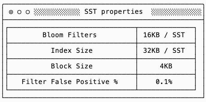
Examples throughout this post assume that SSTs have the following properties (for more details on what these mean, see the previous post on SSTs):
a simple log
The easiest way to work around the immutability limitation of SSTs is to just write new ones.
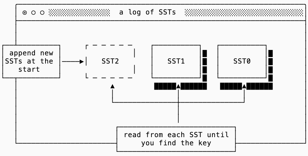
A log index structure continuously prepends new SSTs to the head of the log. When finding a key within the log, a scan is performed sequentially on each SST until the key is found.
write amplification
This structure is surprisingly versatile. The main benefit is that there is no write amplification: rows that are written to a log of SSTs are written exactly once and never rewritten. You pay for this structure with both read and space amplification.
read amplification
The read amplification for a log is the number of bytes you need to read before you find your key. Since the log is structured by time, you know that the first SST in the log that contains your key is the most recent version of it. Assuming you have an empty cache and the SST containing key is the n-th SST, you can estimate the number of bytes you will need to read in the worst case:
  N * sizeof(bloom_filter)
+ (N - 1) * bloom_filter_fp_rate * sizeof(index + block_size)
+ sizeof(index + block_size)
This formula explained in words: you need to read bloom filters for every SST, you will need to read the index + block_size to verify that the key is not in an SST for every false positive, and then read the index + block_size for the SST that contains the final key.
This means that the cost of reading data grows linearly with the number of SSTs.
If you get unlucky and the key you have is old, you can see how this quickly adds up (assuming the “real” data you want to read is a single 1KB row):
Read Amplification with 0.1% False Positive Rate
(Bloom: 16KB, Index+Block: 36KB)

Read Amplification by SST Count (1KB rows, 0.1% FP bloom filters)

  SSTs |   Total Read |     Amp
-------|--------------|--------
    10 |       196 KB |    196x
   100 |      1.64 MB |  1,679x
  1000 |      16.1 MB | 16,486x
The dominating portion of that table are reading the bloom filters. This is why production databases aim to maintain the bloom filters and indexes of all frequently accessed SSTs in memory. It would drop the disk-read amplification by orders of magnitude (though as you have more SSTs in a log-like system the memory pressure for this would be infeasible).
space amplification
This gets us to the space amplification of the log structure. Since we never delete or merge SSTs in a log (more on that later), any SST that contains a duplicate key will have garbage data. How much you pay in space amplification with your log depends on your use case: some (like an audit log use case) would pay nothing since you never overwrite entries, others can pay a significant price.
This is a good time to introduce the concept of a tombstones. How do you delete data if SSTs are immutable? The answer is to, ironically, write more data. If I have an SST 0 on disk that contains keyA -> valueA, I could write a new value in SST 1 that contains keyA -> [deleted]. When I follow my algorithm for “find first instance of keyA in the database”, I’ll find [deleted] in SST1 and know that I should not continue looking in SST 0.
As you can tell, deletions and updates cause more disk space amplification in a naive log system.
eager merge
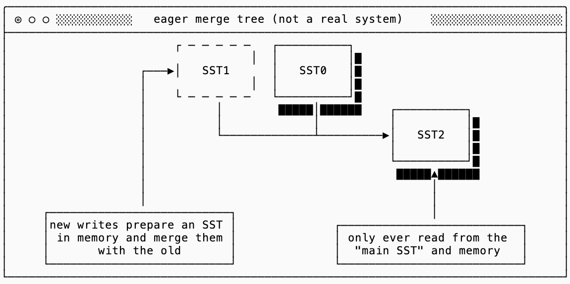
I have yet to see a production system that exhibits this behavior, but it’s interesting to illustrate the polar opposite of a simple log. I’m calling this an “eager merge tree”, a data structure that will always merge any new SST with the old SST as soon as its written into a new merged SST. This works around the immutability by constantly rewriting the old data and discarding it:
read amplification
This system is ideal for reads. You only ever load up the single SST that is on disk, check the Bloom Filter, verify in the index and read the appropriate block. Assuming your single bloom filter and index are in memory (which they would be, since every query reads the same ones) you read a total of 1 block for your key. Using the same parameters as before, that’s a 4KB read for a 1KB key or a 4x read amplification.
space amplification
This system is excellent for steady-state space amplification. You only ever have a single SST on disk, so there’s no garbage data maintained. Compaction is also memory-efficient since you hold one block from each input SST at a time, interleaving them and writing out new blocks as you go.
The catch is temporary disk space during compaction. You can’t delete the old SST until the new merged SST is fully written and synced to disk or a crash mid-compaction would lose data. This means you briefly need 2x your data size in disk space every time you compact. For a 1TB dataset, you need 2TB of disk available even though you’ll only use 1TB in steady state2.
In other words, you need to over-provision your disks to keep steady state utilization below 50%.
write amplification
I’m certain you saw this coming. The eager merge tree is so atrociously bad from a write amplification perspective that it becomes infeasible for all but effectively immutable data sets. Every time you write a new SST and merge with the old one, all data is read and rewritten.
Eager Merge Tree: Write Amplification
(4GB buffer, 1 MB/s writes, 1KB keys)

Data Size | Logical Writes | Physical Writes |   Amp (x)
----------|----------------|-----------------|----------
     4 GB |           4 GB |            4 GB |        1x
    40 GB |           4 GB |           40 GB |       10x
   100 GB |           4 GB |          100 GB |       25x
   400 GB |           4 GB |          400 GB |      100x
     1 TB |           4 GB |            1 TB |      250x
     4 TB |           4 GB |            4 TB |    1,000x
    10 TB |           4 GB |           10 TB |    2,500x
There is almost a brutal simplicity to this: even at 400GB, every 4GB of new data costs you 100x write amplification. Your SSDs won’t last long with this strategy.
log structured merge trees
Let’s build intuition for LSM trees by exploring the middle ground between the two extremes of logs and eager merging. The log based approach shows us that the read amplification is proportional to the number of SSTs. The eager merge approach fixes this, but introduces significant write amplification caused by repeatedly merging small new SSTs with a single large “main” SST.
We could start searching for a middle ground by increasing the size of the “small new SST” before merging it with the main one in an eager-tree. If my dataset is 1GB, I can improve my write amplification by by buffering larger “new” SSTs before merging them:
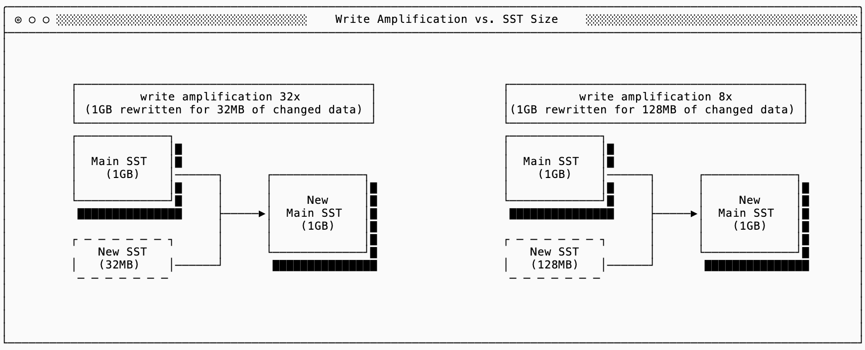
Assuming the new SST only updates existing rows so the new compacted “main” SST is the same size as the old one, you can see that the write amplification is improved the more data I buffer up before compacting. This improvement is helpful but still limiting. Buffering more data before flushing it out causes increased memory pressure and doesn’t help you if the size of your main SST continues to grow.
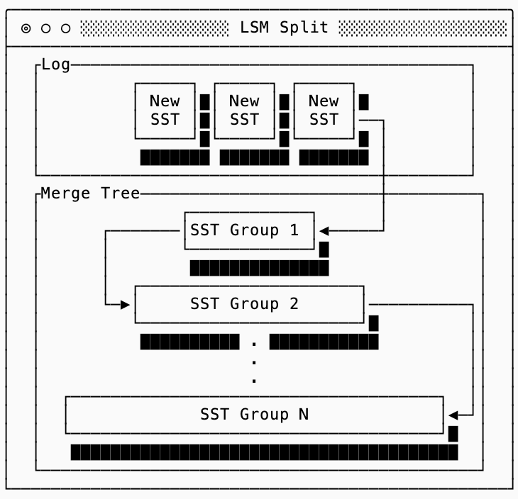
The main insight of an LSM tree is that it provides a continuum between the log and the eager merge structures by maintaining a log for the most recent data, and then “levels” of merged data that increase in size to keep amplification manageable.
SSTs from new writes to the database go into the log. Then you maintain a series of groups of SSTs where each group is larger than the previous group by some multiplier. You can then trade off read and write amplification by tuning the multiplier or the number of SSTs you allow to accumulate in a group.
Before we dive into the specifics of how these trees are structured, there are some common concepts that are shared between all of them:
A level of a tree is typically referred to as
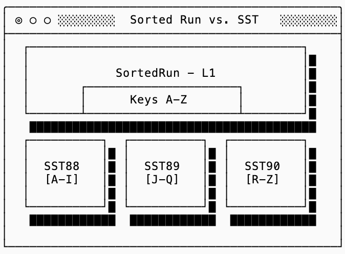
LN(e.g.L1), with the number representing the depth of the tree. In other wordsL0contains the most recent data, and data sinks downward toL1, L2, ...over time through compaction. Note that if you think of trees in terms of “height” instead of “depth” you’re going to trip over the number scheme. I recommend you disabuse yourself of that notion whenever dealing with LSM trees.A sorted run is a set of SSTs that do not overlap in keys, but together cover the entire keyspace. In other words, if Sorted Run 100 contains SSTs 101, 102 and 103 then those SSTs might cover keys
[a-g],[h-m],[n-z]respectively (you would not find a key that starts withkin SST 101 or 103, only in SST 102). These are useful because they allow you to maintain smaller filters and indexes for each SST while using the min/max to find the right SST within a sorted run.
leveled trees
A discussion of LSM trees usually starts with Leveled Trees, since this was their first widely used implementation with LevelDB from Google3. The structure of a Leveled Tree looks like this:
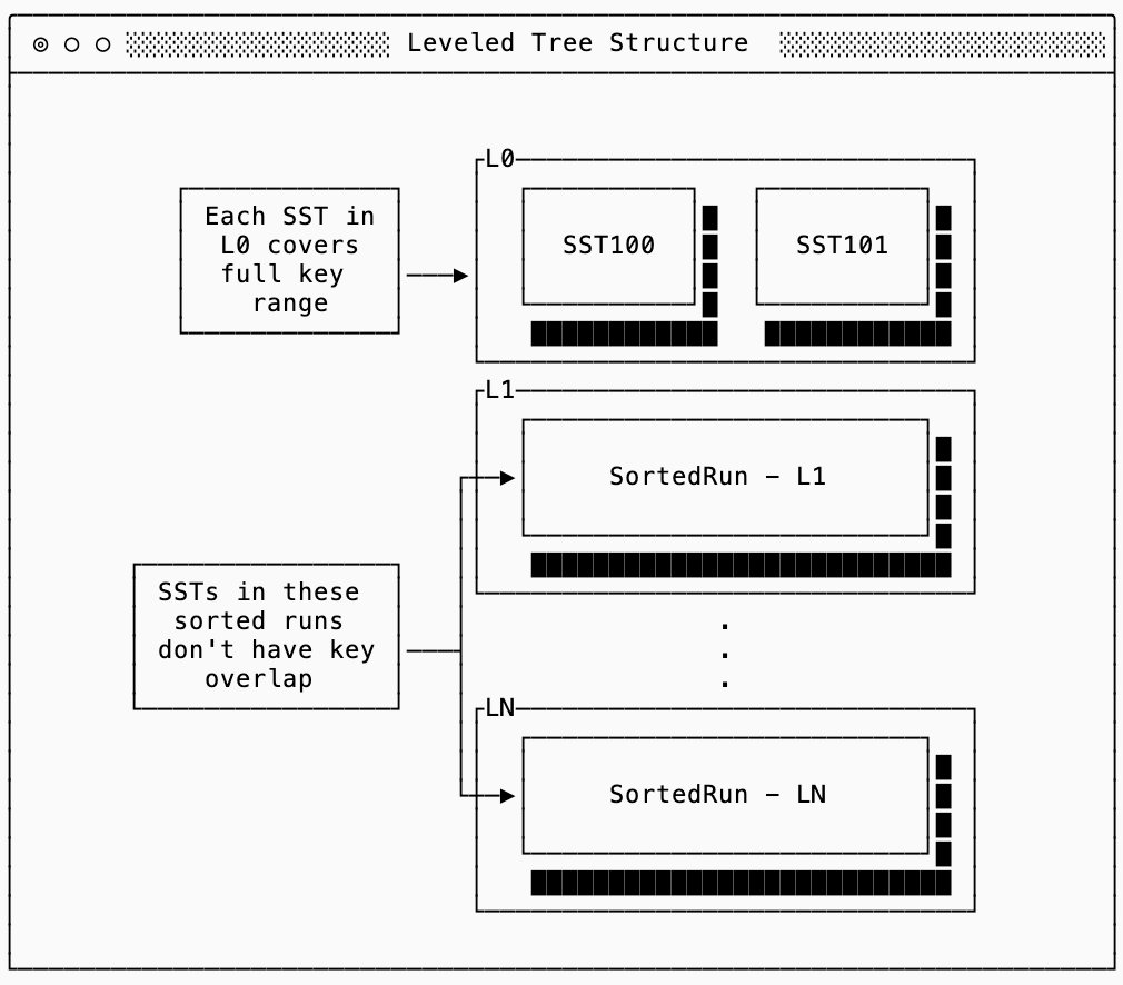
The first level (L0) is special4: each SST in L0 covers the entire key range. In the diagram above it’s possible that key foo exists both in SST100 and SST101. Every deeper level in the tree (L1+) is made up of sorted runs, each of which are split into SSTs with non-overlapping keys. In other words, if the Sorted Run for L1 is split into three SSTs (with ids 88, 89 & 90) then a key that shows up in SST88 is guaranteed not to show up in SST 89 or 90:
The algorithm for making this happen is called Leveled Compaction, and it looks a lot like a combination of the two “naive” strategies covered previously. New writes go into a simple log structure by just appending new SSTs into L0. This allows a Leveled tree to accept writes quickly without paying any cost for compaction.
Then in order to improve read performance, L0 is periodically compacted when it accumulates too many SSTs. Since L0 files can overlap with each other, compaction typically selects multiple L0 files and merges them with any overlapping SSTs in L1 (if any exist). The output is a set of new, non-overlapping SSTs that are placed into L1.
When a deeper (L1+) level exceeds a configured size (configured as a multiple of the previous size to keep the sizes growing exponentially, 10x is common), one or more SSTs are selected and merged with the overlapping SSTs from the next level down. This cascades as needed: if the new level exceeds its size limit, some of its SSTs will be merged into L2 (10x larger than L1), and so on until the tree stabilizes.
read amplification
Leveled compaction’s main point contribution over a simple log is to improve read amplification by bounding the number of SSTs you need to check. For L0, you still need to check every SST since they can overlap, but deeper levels only need to check at most one SST. This means the worst case lookup is:
L0_count * sizeof(bloom_filter)
+ num_levels * sizeof(bloom_filter)
+ bf_fp_rate * (L0_count + num_levels) * sizeof(index + block_size)
+ sizeof(index + block_size)
Assuming nothing is kept in memory (which is unlikely, but helps illustrate the point) we can compare a leveled tree to a simple log when it comes to read amplification:
Read Amplification: Leveled vs Simple Log (10x ratio, 4 L0 files)

Data Size | Levels | Leveled |  Simple Log
----------|--------|---------|-------------
     1 GB |      4 |  160 KB |      196 KB
    10 GB |      5 |  176 KB |    1,640 KB
   100 GB |      6 |  192 KB |   16,036 KB
     1 TB |      7 |  208 KB |  160,036 KB
    10 TB |      8 |  224 KB |    1,600 MB
The leveled tree’s read amplification grows logarithmically (one bloom filter per level) while the simple log grows linearly (one bloom filter per SST).
space amplification
Alongside with read amplification, Leveled compaction improves on both naive designs on space amplification. There’s very little garbage data because (a) SSTs in each level has no key overlap and (b) compaction aggressively merges data downward.
Roughly 90% of your data lives in the last level (assume 10x ratio). This means that in the worst case when the entire remaining tree are updates to the last level, the garbage in the tree is still only 10% of the data size (space amplification is ~1.1x).
Temporary disk space during compaction is also well-bounded. Unlike eager merge, which rewrites the entire dataset and needs 2x disk space, leveled compaction only rewrites the SSTs involved in a single compaction. You need enough headroom to hold the old and new SSTs simultaneously, but that’s a small fraction of your total data rather than all of it. To summarize the comparison:
                   |  Leveled Tree  |  Simple Log  |  Eager Merge
-------------------|----------------|--------------|-------------
Disk overhead      |         ~1.11x |       1-10x+ |       ~1.0x
Memory overhead*   |   logarithmic  |       linear |    constant
Temp disk space**  |     ~11 SSTs** |          0%  |       ~100%

*  Bloom filters + indexes scale with SST count
** Space for old + new SSTs during a single compaction; multiple
    concurrent compactions would increase this proportionally
write amplification
Hopefully you’ve been paying attention, so before you read this section take a step back and guess what you think the write amplification behavior of a Leveled Tree is (generally, compared to a simple log).
If you applied the RUM conjecture to guess that this is where the cost comes in, you are right! Every time data compacts from one level to the next, it gets rewritten. Because each level is 10x larger than the previous, data from the smaller level must merge into the larger one about 10 times before the larger level crosses its size threshold and compacts down.
To determine the write amplification, we want to know how many times a key get rewritten at each level. On average, a key will arrive halfway through the level being filled out, so it gets rewritten about 5 times before moving to the next level. This leads us to estimate the write amplification:
write_amp ≈ num_levels × (size_ratio / 2)Leveled Tree: Write Amplification
(10x level ratio, 1KB rows)
Data Size | Levels | Expected Write Amp*
----------|--------|---------------------
1 GB | 3 | 15x
10 GB | 4 | 20x
100 GB | 5 | 25x
1 TB | 6 | 30x
10 TB | 7 | 35x
* Actual may be lower because not all data makes it to the deepest level, and compaction selection tries to minimize overlap.
While this is way worse than the simple log, it is many times better than the strict eager merge strategy. For read-heavy workloads leveled compaction is often worth it.
size tiered trees
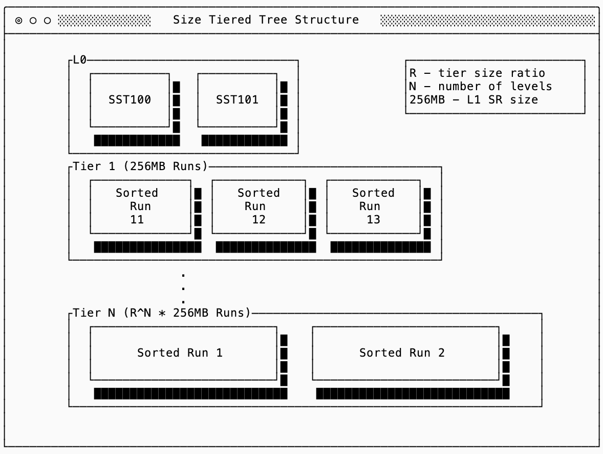
The second main type of LSM compaction strategy attempts to improve with respect to write amplification of a Leveled Tree at the cost of read amplification. The main innovation with size tiered trees is that each tier (the analog to a Level in Leveled Compaction) can have multiple sorted runs which are never partially modified. This is more similar to having each tier be its own “simple log”, periodically compacting an entire section of that log down into the next tier.
In the diagram below, you can imagine that Sorted Run 11 was created when 4 L0 SSTs each of size 64MB were ready to compact. The next four created Sorted Run 12 without touching 11 at all. When there were 4 sorted runs in Tier 1 they are merged together into a new sorted run in Tier 2 with size 1GB, so on and so forth until they’ve merged their way down to Tier N.
write amplification
A good description of the comparison between the two comes from the RocksDB documentation, so I’ll paraphrase that here:
In size tiered storage, new writes move entries from a smaller sorted run to a much larger one. Every compaction is likely to make the update exponentially closer to the final sorted run, which is the largest.
In leveled compaction new writes are compacted more as a part of the larger sorted run where a smaller sorted run is merged into, than as a part of the smaller sorted run. As a result, in most of the times an update is compacted, it is not moved to a larger sorted run, so it doesn’t make much progress towards the final largest run.
If each tier merges R sorted runs into one larger run, then a key is rewritten approximately once per tier. This yields:
write_amp ≈ number_of_tiersOr, using the same assumptions as before, here’s a write amplification comparison between a Size Tiered and a Leveled Tree, which you can see is about an order of magnitude of an improvement:
Write Amplification: Size-Tiered vs Leveled

Data Size | Tiers | Tiered WA (≈ T) | Levels | Leveled WA (≈ L×5)
----------|-------|-----------------|--------|---------------------
     1 GB |     3 |             ~3x |      3 |                ~15x
    10 GB |     4 |             ~4x |      4 |                ~20x
   100 GB |     5 |             ~5x |      5 |                ~25x
     1 TB |     6 |             ~6x |      6 |                ~30x
    10 TB |     7 |             ~7x |      7 |                ~35x
read amplification
And as expected, the order-of-magnitude improvement in write amplification is paid for in read amplification. Unlike leveled compaction, size-tiered compaction does not enforce a single sorted run per tier. Instead, each tier may contain up to R overlapping sorted runs (where R is a configurable merge threshold). In the worst case, a point lookup must check all runs in every tier before determining whether a key exists.
The worst-case read cost becomes:
(N × R) * sizeof(bloom_filter)
+ bloom_filter_fp_rate × (N × R) * sizeof(index + block_size)
+ sizeof(index + block_size)
This grows logarithmically with data size (like leveled), but multiplied by R. Compare:
Strategy    | Read Amplification
------------|-----------------------
Naive log   | O(data_size)
Size-tiered | O(R × log(data_size))
Leveled     | O(log(data_size))

Read Amplification: Size-Tiered vs Leveled
(nothing in memory) - 4 L0 SSTs

          |       |          SSTs |            Reads
Data Size | Depth | Tiered / Level| Tiered   / Leveled
----------|-------|---------------|----------------------
     1 GB |     3 |        12 / 7 |  ~240 KB /  ~148 KB
    10 GB |     4 |        16 / 8 |  ~320 KB /  ~164 KB
   100 GB |     5 |        20 / 9 |  ~400 KB /  ~180 KB
     1 TB |     6 |       24 / 10 |  ~480 KB /  ~196 KB
    10 TB |     7 |       28 / 11 |  ~560 KB /  ~212 KB
space amplification
Size Tiered Trees sit somewhere in the middle between a simple log and leveled compaction for their space amplification requirements. Because sorted runs overlap in key space, obsolete versions and tombstones can accumulate within a tier until a full merge happens. In the worst case, each tier can contain up to R copies of the same key (one per run), but in practice real workloads tend to do better than this.
time windowed structures
The last main type of tree structure commonly seen in LSM trees are time-windowed ones. They are worth an honorable mention because they serve as an “asterisk” on the RUM conjecture: if you know that a workload follows certain patterns, you can improve all three of read, write, and space amplification characteristics. If the assumptions are violated, however, you pay a steep price in either correctness or by rewriting the entire dataset in a major compaction.
Time-Windowed Compaction Strategy (TWCS) works by assuming that data arrives roughly in time order and that there is a practical bound on how late a write can arrive. With this simplification, the database is split into two parts: a mutable region for the current time window and a set of immutable regions for historical windows. New SSTs are written into the current window, and once a window closes, it becomes immutable except for compactions within that window.
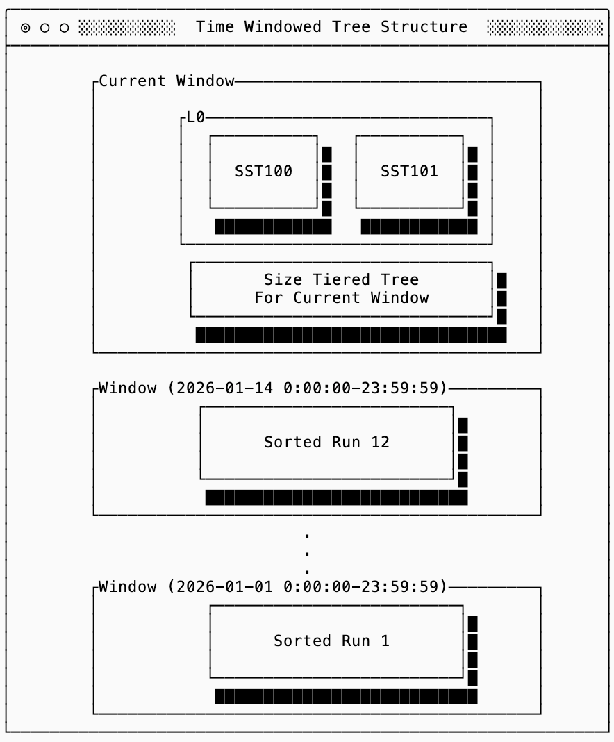
This improves read amplification (assuming reads are also time-scoped) because queries can skip entire historical windows instead of scanning the full tree. It improves write amplification because data does not “bubble down” through progressively larger structures; once a window is sealed, its data is never merged with newer data again. Finally, because compaction is restricted to occur within a single window, both steady-state and temporary space amplification remain bounded by the size of a window rather than the total size of the dataset.
I’ll keep the discussion on this short for now, since this is already a lengthy post, but if you’re curious about more details there’s an interesting discussion on the original Cassandra JIRA ticket that introduced it.
compact()
That’s it for today! Join us next time for a deep dive on B-Trees and why (I believe) LSM trees are having their moment in the sun for object-storage native systems.
Read and write amplification here is simplified to illustrate the key parts of LSM tree structure. In practice, amplification also accounts for other factors such as the number of IOPs (which may matter more than the amount of data read in situations such as using EBS with limited IOP capacity).
There are strategies for mitigating how much space amplification you need by incrementally deleting old parts of the data while you write new SSTs out.
This was introduced by Jeff Dean and Sanjay Ghemawat, though the initial LSM paper was written by O’Neil in 1996. Personally, my favorite paper on the subject is Dostoevsky.
A “pure” leveled tree would not have an L0, instead it would flush merge data directly into the lowest level of the tree. In practice, this is often too expensive so leveled trees treat the top level similar to a log. See the next section for more details.
Excellent deep dive into the amplification tradeoffs. The size-tiered vs leveled comparsion makes the RUM conjecture super tangible because seeing the order-of-magnitude differences in write amp really clarifies why systems like Cassandra and RocksDB make such different choices. I debugged a production issue once where understanding that leveled compaction was rewriting data ~30x helped us shift to a more suitableengine.
Read amplification and write amplification must
also be measured in number of IO requests and
not just in relative data volumes.