frameworks for understanding databases

building mental models for tradeoffs in performance, availability and durability in data systems

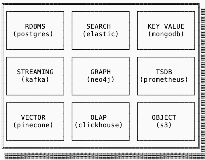
There are nine types of online databases: relational, key-value, time series, graph, search, vector, analytical, streaming, and object. This blog series is for engineers that want to learn more about how these systems work underneath the hood.

This introductory post first presents a mental model for understanding data system tradeoffs and then outlines the common building blocks. We’ll follow this up with deep dive series on each of the nine data systems types¹.

the mental model

All databases have one purpose: to store data so you can retrieve it. This core similarity means that, if you squint, all databases look similar. Evaluating them becomes a question of understanding tradeoffs that can be made.

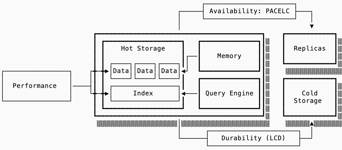
I evaluate data systems on three dimensions, and evaluate each of those dimensions with a set of frameworks (we’ll dive deeper into these throughout the post):

1. For reasoning about performance the Read, Write and Space Amplification of a system determine how much work is done on query, ingest and compaction respectively. Then, the indexes and data orientation are evaluated with the RUM conjecture.

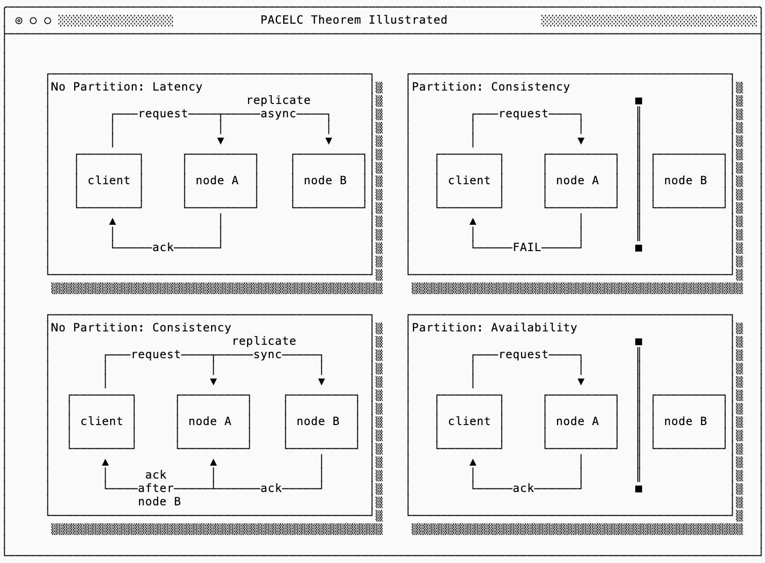
2. For reasoning about availability in a distributed system, the PACELC framework is an evolution of the widely referenced CAP theorem. In steady state, you trade off between latency and consistency — only during a network partition do you choose between availability and consistency.

3. For reasoning about durability (especially in cloud native systems), the LCD framework illustrates that you may pick two of Latency, Cost and Durability.

Usage of these frameworks answers how to choose a data system that serves your use case at the acceptable cost (both on hardware requirements as well as operational overhead).

performance

framework

There’s the famous Latency Numbers Every Programmer Should Know chart² from Jeff Dean that helps reason about why I/O efficiency is so important.

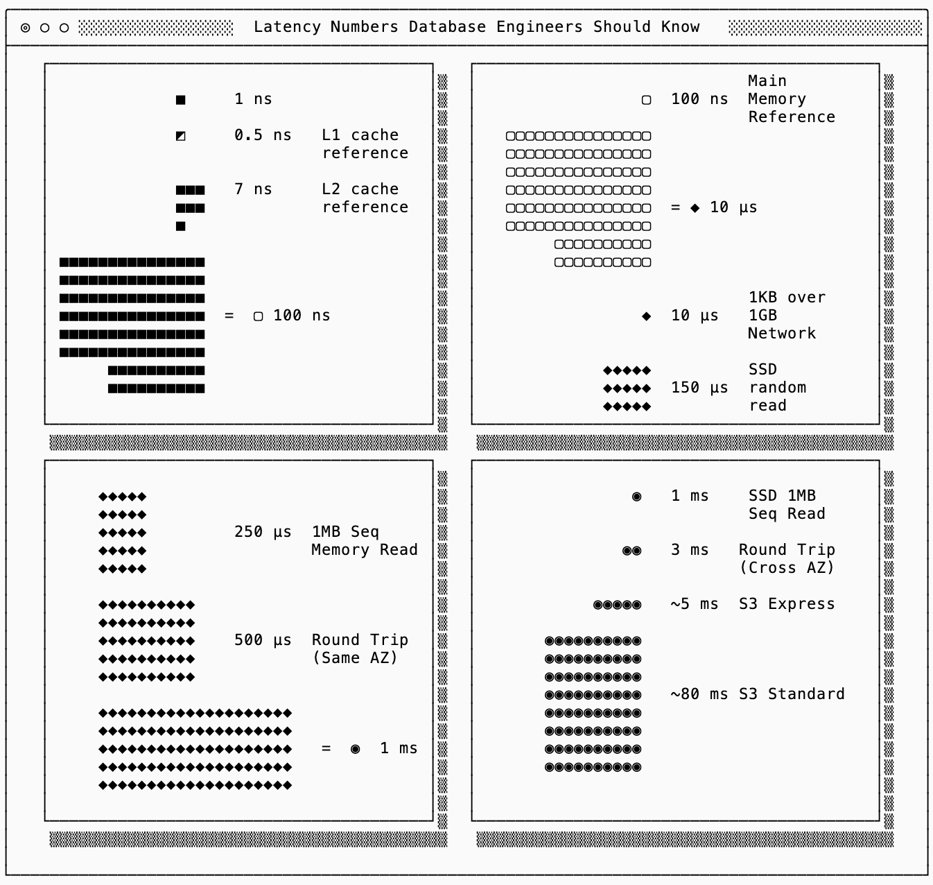
The goal of a data systems’ storage layout is to (a) ingest data into a durable medium as fast as possible and (b) get required data to serve a query into L1 cache as fast as possible. Sometimes that data is already there, other times is on the disk of a machine in another AZ. The latency cost of fetching the latter dominates system performance.

Different systems make tradeoffs on read, write and space amplification:

1. Read amplification measures how many bytes are required to serve a single logical query. More read amplification happens in systems optimized for write throughput.

2. Write amplification quantifies the overhead when a database writes more bytes than strictly necessary to store a piece of data, often due the index structure or compaction.

3. Space amplification captures the ratio between actual storage consumed and the logical data size, accounting for fragmentation, tombstones, and redundant copies. A good example here is a size of a bloom filter (a large bloom filter can help reduce false positives, but takes up more memory).

indexes

A naive database with no index must scan the entire raw storage, potentially across many machines, filtering out points that don’t match the query. Since this is more data than what can fit in L1, much of that data will be elsewhere.

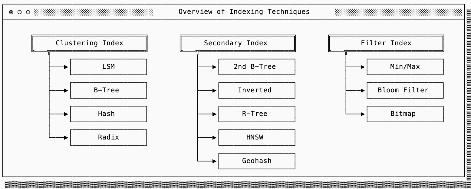
Indexing is the strategy used by data systems to reduce the amount of data scanned. I think about indexes in three categories: primary, secondary and filters.

1. Clustering indexes are how the raw data is organized. For example an LSM Tree (used by SlateDB, Cassandra, etc…) stores the key-values pairs in SSTs, which sort the keys in lexicographical order so a query can binary search to find the required key.

2. Secondary indexes are auxiliary structures that return primary keys³, which can then be used to lookup the raw data. For example, an inverted index (used by Lucene) will return a list of primary keys that contain a particular value (this is particularly useful in search use cases).

3. Filter indexes are often embedded within the primary index to help filter out blocks of data. You’ve likely heard of bloom filters (used by SlateDB, Clickhouse, etc…), which can guarantee that a key you are attempting to lookup does not exist in a particular block of data.

I reference the RUM conjecture when evaluating indexes. This grounds the discussion with the understanding that a single index structure cannot be optimized for read, update AND memory overhead simultaneously. In other words, indexes tradeoff across read, write and space amplification to improve performance of reads, updates or memory utilization.

data orientation

The previous section discussed how the index layout affects how fast you can get data into L1 cache, this section discusses the raw data format and its impact on the types of computations a system can execute.

The primary difference between the way databases store raw data is the way that data is oriented: row or columnar. If your workload reconstructs complete rows choose a row-based data system. If your workload aggregates values across rows choose a columnar system.

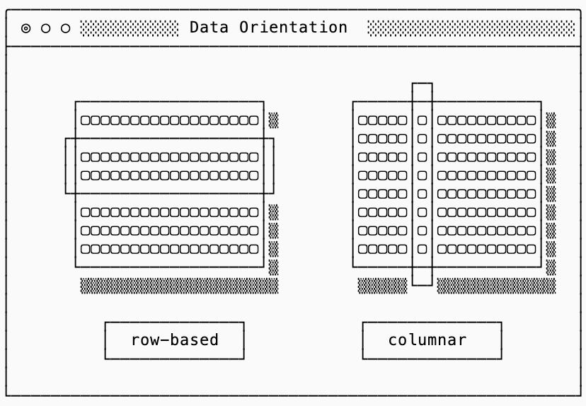
Why? In a row orientation, the entire value for a single row is stored in one place, but aggregating across rows for a few columns means reading unnecessary data. In a column orientation, values across all rows for the same columns are stored in one place, but reconstructing an original row means reading unnecessary data.

Data orientation directly impacts read amplification. To illustrate, consider rows of 16KB with 32 columns of 500B each stored in blocks of 64KB. In a row-based system, fetching one row reads a 64KB block but discards 48KB of unnecessary data (read amplification of 4x). In a column-based system, fetching that same row requires reading 32 separate 64KB columnar blocks and discarding ~2MB (read amplification of over 100x). The opposite is true when aggregating columns across multiple rows.

Beyond minimizing read amplification, aligning data layout with workload patterns enables optimizations like vectorized operations (SIMD) in columnar systems, which are only possible because each loaded memory block is a single-typed array.

compaction & garbage collection

Compaction and garbage collection (GC) are common strategies for reducing write amplification in favor of read/space amplification. A data system can only write a single block at a time, which means that if the contents of that block are modified it is no longer entirely valid. Since rewriting a block in-place may be impossible due to fragmentation, the strategy most systems use are to append new blocks that model updates to the old blocks.

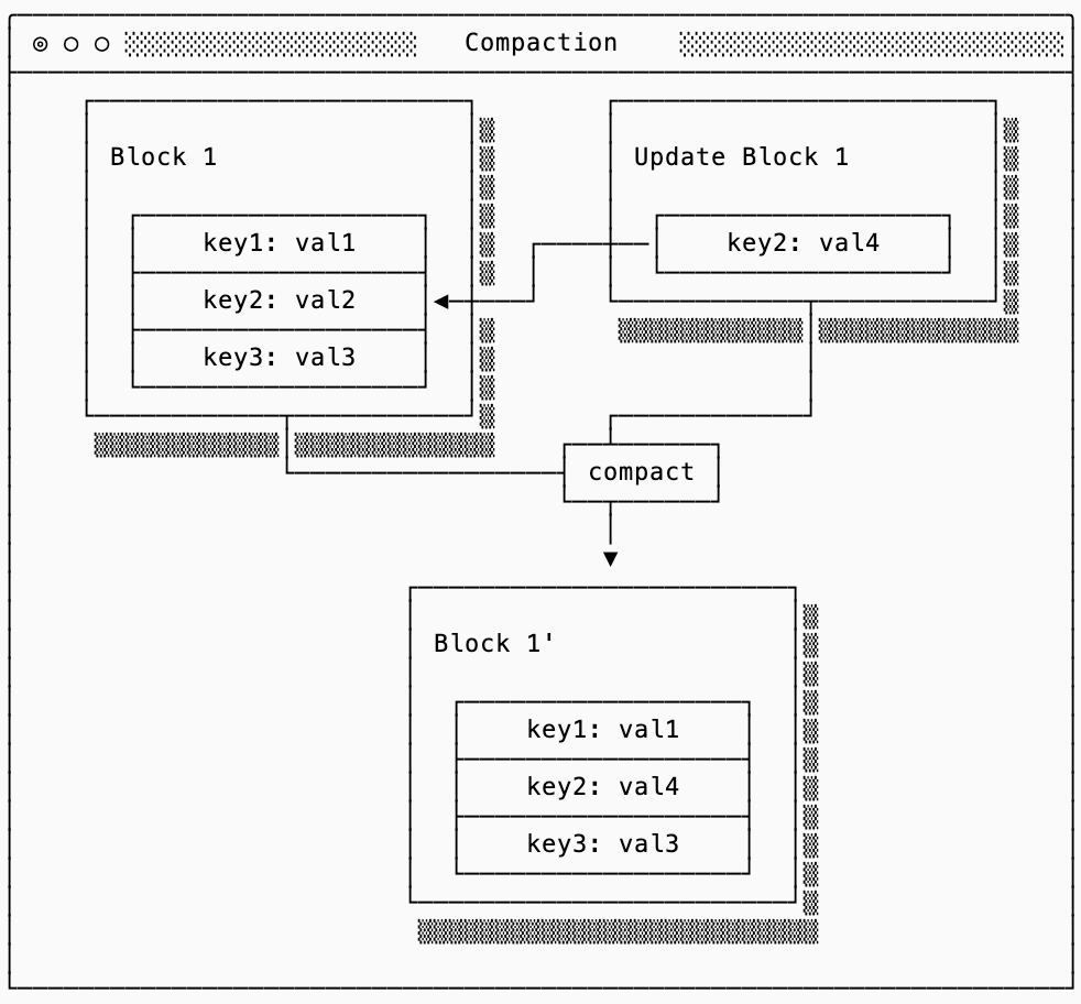
Compaction takes files that have overlapping data and compact them back into files with non-overlapping data. These compactions jobs don’t immediately need to clean up the old files that are still sitting around. Garbage collection can run separately, cleaning up orphaned files. This separation allows keeping “backups” to old data.

availability

framework

Few applications need more than 3 nines of availability (~9h of downtime yearly) because downtime violations in excess of that frequently occur as the result of human, not machine, failure.

Despite this, more availability is always better so unless your system falls into the small select group of requiring high availability (HA) it becomes a cost tradeoff: how much does a minute of downtime cost compared to the overhead of operating with HA.

To make sense of tradeoffs in HA systems, I recommend you read up on PACELC, but the summary is that during a network partition the CAP theorem applies, but otherwise you tradeoff between consistency and latency.

system architecture

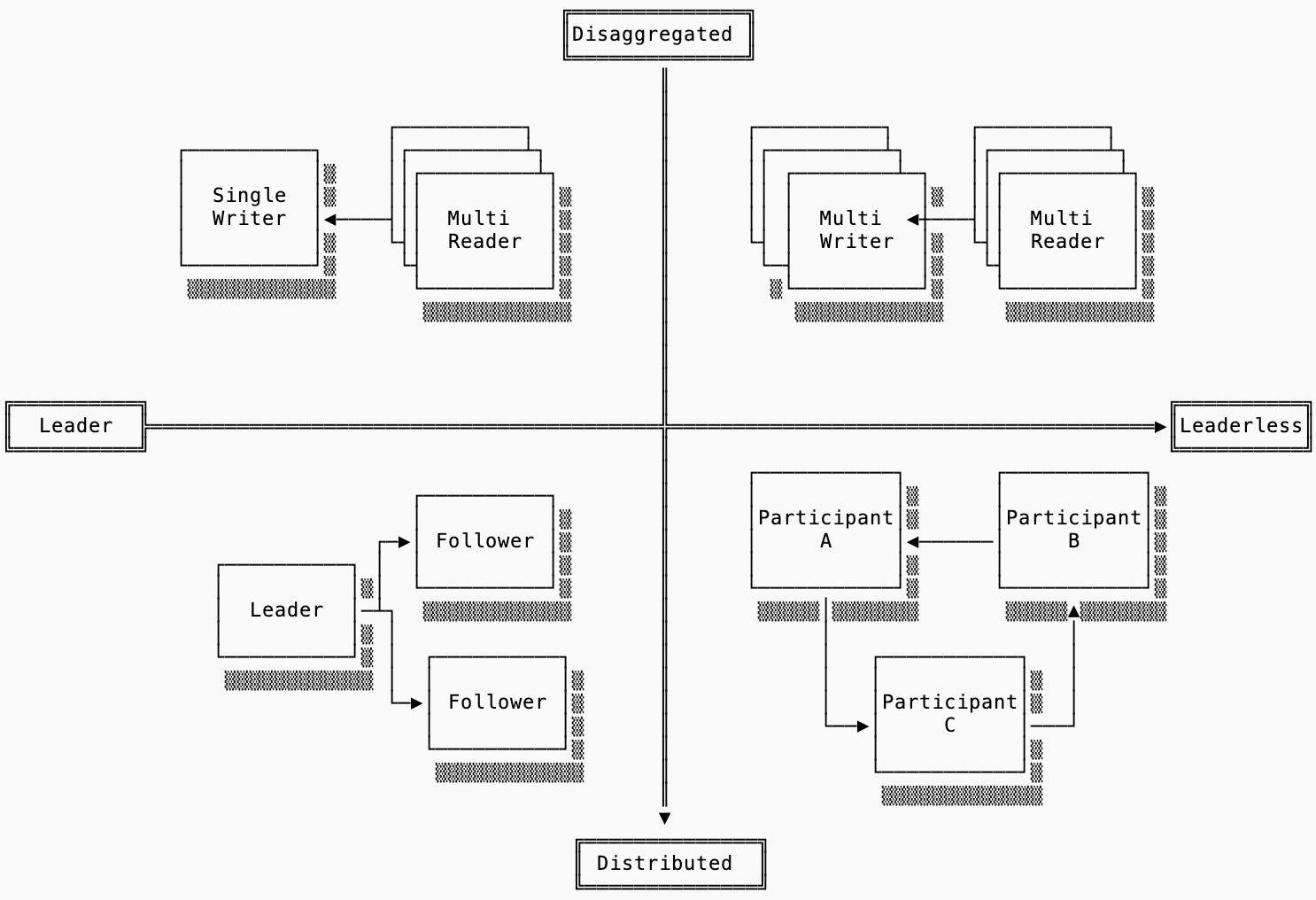
Availability in systems is tied to the system’s deployment architecture. Consider the two-dimensional matrix below. The first axis is the leader/leaderless dimension which models whether or not all writes must be funneled through a single node. The second axis is the disaggregated/distributed dimension which models whether replication is done within the system or delegated to a separate (typically object storage) system:

1. Single Node Deployment: omitted from the diagram above is a non-HA deployment strategy that makes sense for some data systems like caches and edge database deployments. Example: sqlite

2. Single Writer, Multi-Reader: a single-node system with the additional feature of writing to shared storage (e.g. S3) so other readers can read it. Example: slatedb

3. Multi-Writer, Multi-Reader: a deployment mode that allows for writes and reads across many nodes, typically resulting in a async coordination layer. Examples: warpstream, quickwit

4. Leader / Follower: a distributed system that requires writes to go to a single leader, which will replicate to followers before acknowledging the write. Example: kafka

5. Leaderless: this is a distributed system that can accept writes to any machine, but will still replicate to other nodes in the cluster. Example: scylla

The left half of the quadrant prioritize consistency. Since valid writes will only be handled by a single machine, it is easier to provide ACID semantics. Single-writer systems are always consistent, but allow trading off latency for durability (see next section). Leader-follower systems allow configurable consistency by reducing the number of acquired acks from followers. Both systems experience downtime in the event of a writer or leader failure.

Leaderless systems prioritize availability, since a single node failure does not require a leader election process or a new writer to restart. Consistency, on the other hand, requires increased latency because all writes must meet quorum.

durability

framework

The primary consideration for durability is a tradeoff between latency, durability and cost. You can see the durability guarantees of each of the following durability strategies in the chart below:

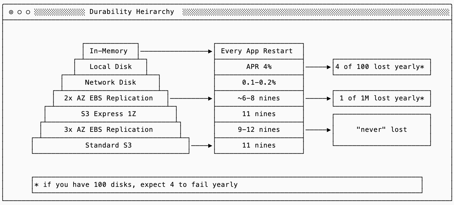
If you keep data only in-memory on a single node, you have no durability. When you fsync that data to a local disk, you gain a bit more. When you replicate that to a network disk (EBS) or across multiple zones, you get more with each step.

In coupled storage and compute systems, durability was more closely tied to availability. If you were running with 3 replicas across zones and prioritized consistency then you had three nodes that potentially had the data in memory, making durability of the storage a slightly less important concern. In a disaggregated system you no longer replicate within the compute subsystem and delegate that to object storage, the tradeoff becomes more acute.

storage options

Once you’ve made your decision on how durable your data needs to be, the next choice is where to store durable data. The chart below shows the latency and cost deltas between different solutions:

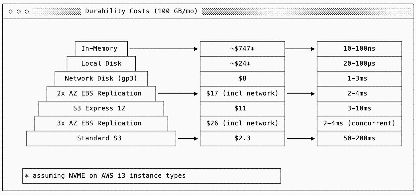
It is possible to have a tiered write system: recent writes can go to a faster storage solution and eventually tier to the slower solutions. This is an example of the LCD tradeoff: if recent writes go to local disk, they can be fast (and cheaper than in memory) but are less durable to an outage.

WAL (write ahead log)

Write ahead logs (WALs) are a strategy that illustrate the tradeoffs of both the LCD and RUM conjectures. Data systems will write changes to the database in a write-optimized format (effectively logging the request with no transformations) to a durable storage. Using the LCD framework, WALs increase cost (by increasing write amplification) so that writes can be durable with lower latency. WALs are also an extreme example of UM data structures (update & memory optimized), but reading from them is inefficient and reserved for failure situations.

fysnc()

That’s it for today folk! I hope this has helped shaped the way you understand and evaluate different data systems. Next time, we’ll pick up key value stores as the first data system we’ll examine in more depth to see how we can apply this framework to a specific type of database.

1. If you can’t wait, I highly recommend Designing Data Intensive Applications. It’s a phenomenal book that covers a bunch of core database concepts. If you can wait a little bit, the second edition is coming out soon and is likely to be updated with important additions.

2. I’ve modified the latency numbers chart to have some important cloud-native latency numbers, such as S3/S3 Express and removed less relevant numbers.

3. Often secondary indexes will point directly to the block of data containing the corresponding row instead of just the key, which saves one lookup but requires more index maintenance when the data changes (nonfunctional updates to the data layout, such as compaction, require modifying such indexes).