sorted string tables (SST) from first principles

why sorted string tables are the swiss army knife for data systems and how they are implemented

This blog is about how data is laid out on disk, specifically about the details of Sorted String Tables (SSTs). Let’s cut to the chase.

SSDs and memory

First, it’s important to understand how data gets from disk in to usable memory. Most cloud instances use SSDs, so we’ll focus on that instead of spinning disks.

If you haven’t read the initial frameworks blog post of this series I recommend starting with that. In this context, the main point to takeaway is that not all read amplification is created equal. All databases need to abide by the laws of physics: fetching data that’s already in memory is hundreds of times faster than fetching data from over the network. Data structure design is all about minimizing the amount of data you need to fetch from expensive storage tiers while reducing the memory overhead (this an application of the RUM conjecture).

pages on storage devices

A high performance data system needs to reduce the amount of unnecessary bytes read to serve a query, reading only the necessary (”hot”) data.

An ideal system would read exactly the bytes it needs for the data it wants, but the fundamental unit of I/O isn’t a byte. On SSDs, it’s a page (typically 4KB). This means that whether you request a single byte, a hundreds bytes, or four thousand bytes from your disk you’ll still get the 4KB.

You can verify this on your own machine:

# on MacOS, check the size of the page on your disk
> stat -f %k /
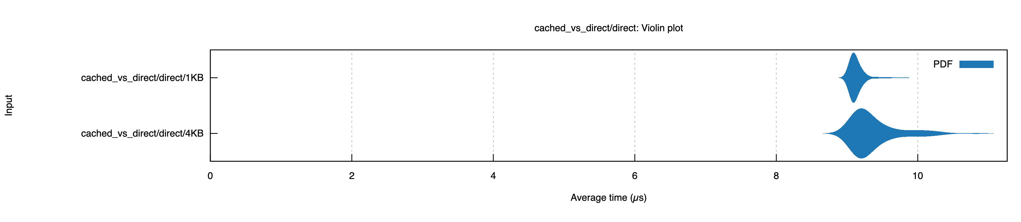
4096

To see this in action, I ran an experiment measuring read latency for 1KB vs 4KB reads using Direct I/O (bypassing the OS page cache). Despite requesting 4x less data, the 1KB reads took about the same time as the 4KB reads (about 9.2µs) on my SSD¹:

Here’s where it gets interesting for database design. Imagine you’re serving a query that needs a single 256B row that lives somewhere in a 4KB page alongside other rows:

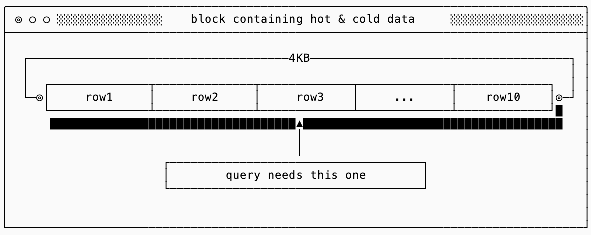
To read row3, you have to read the entire page. Rows 1 through 10 come along for the ride whether you want them or not. The ratio of “data you read” to “data you needed” is an instance of read amplification. In our example, if you needed 256 bytes but read 4KB, your read amplification is 16x. That sounds sub-optimal, but it’s unavoidable given the hardware constraints.

spatial & temporal locality

The read amplification from page size and sizes isn’t all bad news.

There’s a fixed cost overhead to reading a single page from disk. On an SSD the actual data transfer part is less than 1-2% of the total latency (the rest comes from processing the command, translating the logical address to the physical location on the disk, etc…). This means that it takes approximately the same amount of time to read 1 page, independent of whether that block is sized 512B on a 512B system or 4KB on a 4KB system.

To take advantage of the page size, databases attempt to place data that is commonly read together physically close together on the storage device, ideally in the same page. Typically this means one of two things: either the data keys are the similar (spatial locality) or the keys were written around the same time (temporal locality).

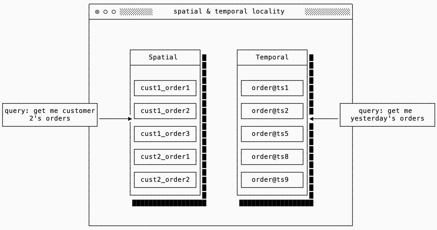
This technique helps reduce the overhead of read amplification that comes from reading data you won’t access. As an example, if I’m executing a query that sums the total cost of orders from a particular customer my query execution path is likely to perform a loop that looks something like:

total = 0
for order_id in [cust2_order1, cust2_order2, cust2_order3]:
	let order := db.get(order_id)
	total += order.cost

If my first call to db.get(cust2_order1) fetches a 4KB page from disk that contains the orders cust2_order2 and cust2_order3 then when I next call db.get(cust2_order2) that data will already be in the OS page cache, which will make it much faster to load.

This is why designing the key for your database is so important. It is the first attempt to make sure that you can take advantage of the spatial locality of the data on disk.

mutability on SSDs & blocks

Unlike hard drives and spinning disks, data that’s written onto an SSD cannot be directly replaced without first erasing that data. The electromagnetic physics behind it is beyond my expertise, but the way I think about it is that while you can write a small (4K) page, you cannot target erasure at that level. Instead, erasure works at a much higher level called a block (typically 128-256KB).

Because of this effect, when you rewrite data on an SSD you are actually writing a new data block and telling the SSD controller (a piece of firmware that comes loaded on your SSD) the new location of the data. Eventually, the controller will erase large chunks of garbage data in a mechanism that looks very similar to handling garbage collection in a memory allocator.

SSDs, therefore, much prefer that pages are not modified over and over again. Instead they become invalid in large ranges at a time. This means that immutable on-disk data structures work well with SSDs and any mutable structure will cause significant write amplification at the hardware level. We’ll get to the implications of this a little more in a future blog post about B-Trees and LSM trees.

For now, we’ll draw the conclusion that immutable storage formats have an edge.

storing data durably on SSDs

To recap the above sections, SSDs push you to use a data structure that:

1. Is written and deleted in large batches aligned to the internal block size (e.g. 256KB)

2. Is immutable to avoid the overhead associated with rewriting data

3. Organizes data in a way that clusters related data together to take advantage of the page size

There are several ways to organize immutable data durably that meet these requirements, the simplest of which is an append-only log. In a log, the system writes records sequentially (aligned to block size) and scans from the beginning for reads. You can see why this works well with SSDs:

1. Logs let you batch data together and write them when you have enough data.

2. Logs are immutable, typically with some retention at which point you drop entire sections of it.

3. Logs organize data in a way that is optimized for the particular read pattern of reading data in the order it was written.

The downside of a log is the performance of random reads: you might need to scan the entire file to find a specific key. Some systems (like BitCask) address this by storing the entire key-set in memory with pointers to the location on disk stored in memory.

To make reads directly from disk efficient without exploding memory usage, you need some other kind of structure. There are a number of different strategies, but for this post I’ll focus on a typical approach used by row-based systems (SSTs).

Sorted String Tables (SSTs) build off the ideas from the log to play well with the limits of SSDs (you’ll see the similarity even further when we talk about LSM trees). If you think of a log as an array sorted on an implicit timestamp key, SSTs are essentially the same structure but sorted on a user-defined key instead. To make this possible, databases that use SSTs first buffer data sorted by that key in memory until they’ve collected enough data to write a large, immutable batch.

sorted string tables (SSTs)

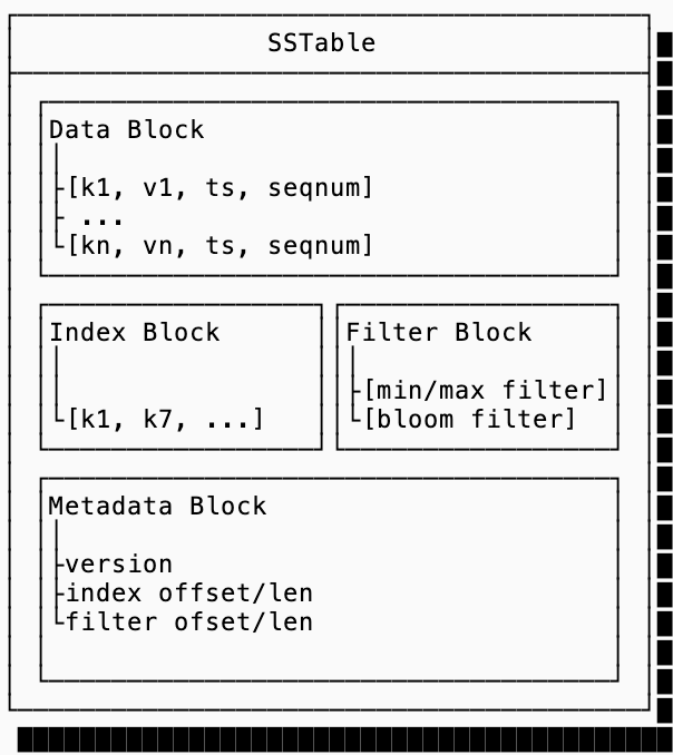
This section will go over the design and implementation of a basic SST: an immutable storage data structure for key-value data. Here’s a reference to look back on that covers the big-picture of an SST layout (this is inspired from the SlateDB SST layout, though other implementations such as RocksDB are quite similar):

data blocks

The core concept of a sorted string table is to store data on disk sorted by the lexicographical ordering of the byte representation of their keys. In other words, a single data block of an SST can be thought of as a byte array constructed like this:

struct Record {
	key: Vec<u8>,
	val: Vec<u8>,
}

struct SstDataBlock {
	data: Vec<Record>,
}

impl SstDataBlock {
    fn from_unsorted(data: Vec<Record>) -> Self {
        let mut data = data;
        // sorts the records by the lexicographic order of the keys
        data.sort_by(|a, b| a.key.cmp(&b.key));
        Self { data }
    }
}

This strategy is nice for two reasons: first, it takes advantage of the spatial locality principle we discussed above. Similar keys are stored next to one another. Second, and perhaps more fundamental, it allows us to binary search the data within an SstDataBlock:

fn find_record(&self, key: &[u8]) -> Option<&Record> {
    self.data.binary_search_by(|record| record.key.as_slice().cmp(key))
        .ok()
        .map(|index| &self.data[index])
}

But this relies on the in-memory representation of the SstDataBlock. We still need some way to get this struct onto disk which only understands simple byte arrays [u8]. There are many strategies for serializing the data block of an SST; production data systems will often use techniques such as prefix encoding for keys and varint encoding for lengths to reduce the amount of space a block takes up but for this exercise we’ll do something simpler: we’ll just encode the block as:

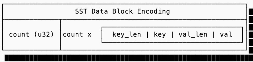
And a code mockup for reading and writing these SstDataBlock instances:

fn encode(&self) -> Vec<u8> {
    let mut encoded = Vec::new();
    encoded.extend_from_slice(&(self.data.len() as u32).to_le_bytes());

    for record in &self.data {
        encoded.extend_from_slice(&(record.key.len() as u32).to_le_bytes());
        encoded.extend_from_slice(&record.key);
        encoded.extend_from_slice(&(record.val.len() as u32).to_le_bytes());
        encoded.extend_from_slice(&record.val);
    }

    encoded
}

fn decode(data: &[u8]) -> Self {
  // decode is more verbose so it's emitted here but it just reads
  // the number of records, then deserializes them one by one reading
  // the length of the key, then the key, then length of the value,
  // then the value itself
  ...
}

indexes

The data block covers how to get a record from within a block, and technically this is all you need for a functioning SST.

Simply storing data as a series of sorted blocks, however, isn’t ideal. If that’s all you did, your query algorithm would end up reading blocks in a binary-search pattern fetching entire blocks to decompressing them just to see whether or not the key you’re looking for is even within the range of the block.

To solve this problem, SSTs introduce multiple layers of indexes.

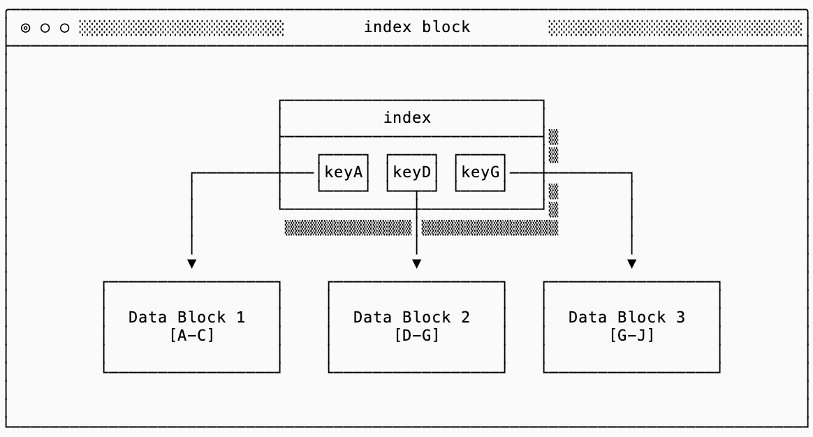
the main index

The first index (often just called “the index”) is a smaller data structure that just contains the first key of every data block and the location of the block (an offset within a larger file). This allows you to load the index into memory and binary search on that, which is an order of magnitude smaller than trying to load the actual blocks, to find the required data block.

To put the index size for corresponding data blocks into perspective, let’s imagine you have 4KB blocks with keys that average 8 bytes (a u64) and values that average 256 bytes. This means a single data block can contain approximately 15 records. The index in the most naive format can contain 512 keys (with delta compression you can squeeze significantly more). If each key is the first key of a block, a 4KB index block can index 2MB of data blocks, or 7680 records.

The code for the index block would look something like this (without the encoding/decoding section, which looks very similar to the data block encoding and decoding):

pub(crate) struct IndexEntry {
    key: Vec<u8>,
    offset: u64,
}

pub(crate) struct SstIndexBlock {
    entries: Vec<IndexEntry>,
}

/// used to find which block in the SST contains the key
/// that you want using the index. once the data block is
/// identified, it should be deserialized into a SstDataBlock
/// and then searched using SstDataBlock::find_record for the
/// exact record
impl SstIndexBlock {
		fn find_entry(&self, key: &[u8]) -> Option<&IndexEntry> {
        match self.entries
            .binary_search_by(|entry| entry.key.as_slice().cmp(key))
        {
            Ok(i) => Some(&self.entries[i]),
            Err(insertion_point) => {
                if insertion_point > 0 {
                    Some(&self.entries[insertion_point - 1])
                } else {
                    None 
                }
            }
        }
    }
}

filter indexes

Up until this point, we made the assumption that all the data you’d need exists in a single SST. We’ll discuss why you might not want that in a future blog post about LSM trees, but for now I’ll ask you to accept that it’s often better to store data in multiple SSTs instead of one big one.

If you setup your storage like that, it is helpful to know whether or not a given SST has the key you’re looking for before you even try reading the index and data blocks. This information is stored in a filter block, and there’s typically two forms of filters that are used: min/max filters and Bloom filters.

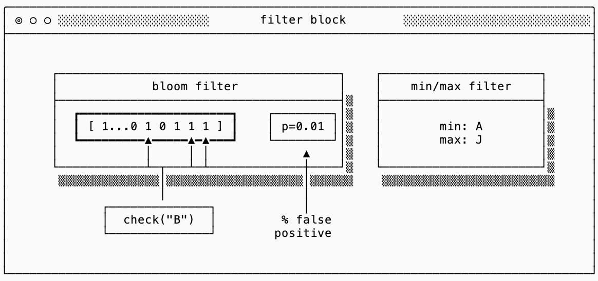
Min/Max filters are extremely simple filters that just encode the minimum and maximum keys that exist in the SST. This very simple data structure takes up very little space and can save a lot of computational work in certain storage systems that lay out their SSTs across very wide key ranges (think using a number such as timestamp as the key).

Bloom filters are more complicated and come with some interesting tradeoffs. There have been many sources that explain how these filters work, if you’re curious the Wikipedia page has an excellent overview. If you’re not, the important thing to understand is that they’re a probabilistic data structure that can tell you with 100% certainty that a key does not exist in SST but it cannot guarantee that a key does exist. Their accuracy is measured by their false positive chance: each false positive means you need to dig into the index and data blocks unnecessarily, finding out that the key in fact does not exist.

index space amplification

Indexes and filters aren’t free and, typically, you want to keep the entire index along with any filters in memory to avoid deserializing indexes over and over again.

The implication is that indexes are a fundamental way to tradeoff between read and space amplification.

To tune between the two, you can change the size of the data blocks (smaller blocks means larger indexes, but less read amplification as less data needs to be paged in). I ran an experiment on RocksDB in practice to show this in action². The experiment set up a data set of 4GB size and varied the block size, checking the total size of the SST (on disk), the size of the index (in memory) and the read throughout.

$ space_amp --block_sizes=4096,8192,32768 --read_ops=50000
Raw payload bytes: ~4GB (33554432 entries)

Block Size    Total SST   Table Mem   Reads/s
4.00KB           3.51GB      38.9MB     13144
8.00KB           3.48GB      19.3MB     11310
32.0KB           3.45GB      4.88MB      9311

This shows what we expect to see: smaller block sizes mean larger indexes, higher memory utilization but faster reads. It also shows the diminishing returns of large indexes. When we decrease the block size 8x, memory grows by approximately the same factor but the read throughput only improved by 1.4x.

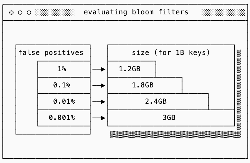
Bloom filters are not exempt from this tradeoff either: to reduce the false positive rate of a bloom filter, you need a large one (more bits). The good thing is that the math to compute the false positive rate is straightforward. Assuming your SST stores 1 billion keys, the diagram below shows the false positive rate and the corresponding Bloom Filter size.

metadata block

The final block in an SST is the metadata block. Despite its humble size, typically just 48-64 bytes, it plays a critical role by storing the offset and length of the index and filter blocks, plus a magic number and version that allows the SST format to evolve over time.

But here’s an interesting question: Why are the index and bloom filter blocks at the end of the file?

The answer reveals a constraint of SST construction. When building a large SSTable you face a choice. Your first option is to buffer the entire SST in memory, build the complete index and bloom filter, then write everything in the “correct” order: index, bloom filter, data blocks. Alternatively, your second option is to stream data blocks to disk one at a time as they’re built, constructing the index and bloom filter incrementally as you go. If you take the second path, then you can’t know the locations of the blocks until the end, so you can’t write out the index block until then.

Note that this optimization only really applies when your data is already in sorted order (such as when merging two SSTs), otherwise you need to buffer the data in memory to sort it in first place.

SSTs are general purpose building blocks

While SSTs are an obvious fit for key-value storage, sorted rows turn out to be a remarkably general abstraction. Almost any access pattern you care about can be encoded into SSTs if you’re clever about how you structure your keys.

The insight is that lexicographic sorting on byte strings gives you hierarchy for free. When your keys share a prefix, they’re stored physically adjacent. This means a “range scan over all keys starting with X” is just a sequential read which is the best possible access pattern for storage devices (remember that the minimum fetch of data from a disk is 4KB, even for an SSD, so if all of that data is relevant then you aren’t paying excess read amplification).

encoding access patterns into keys

There’s a spectrum of cleverness in how you shove data models into key-value form. This section goes through strategies you can use, from obvious to devious:

level 0: plain key-value lookups

The trivial case models the keys exactly the way you are looking them up. There’s nothing clever about this and often this is all you need:

"user:alice" → {name: "Alice", email: "alice@bitsxpages.com"}
"user:bob"   → {name: "Bob", email: "bob@example.com"}

level 1: key namespacing

The next requirement might be to store different types of data in the same SST rather than split each data type into its own SST. To do this, you can prefix your keys with the type of data they represent and then construct your lookup key based on that.

The following example has three key types: metadata keys, users and sessions:

"meta:schema_version" → "3"
"meta:created_at"     → "2024-01-15T00:00:00Z"
"user:alice"          → {name: "Alice", ...}
"user:bob"            → {name: "Bob", ...}  
"session:abc123"      → {user: "alice", expires: ...}

Because keys are sorted, all the meta: keys cluster together, all the user: keys cluster together, and so on. A range scan with prefix user: gives you all users. This is effectively multiple logical tables in one physical SST.

level 2: composite keys for hierarchy

This is when things start getting interesting. You can effectively “decompose” a single complicated key into multiple rows for efficient lookups of both the composite key as well as the single key. Imagine our users had a set of orders, so the logical data would look like:

"user:alice" → {
	name: "Alice", 
	orders: [
		{"id": "7", "item": "catnip", "count": 2},
		{"id": "112", "item": "dog_treats", "count": 11},
	]
}

Using level-0, and level-1 techniques outlined before we could get decently far:

1. Level 0: Store "user:alice" as the key, and include the full order details in the document value (match the logical model)

2. Level 1: Store "user:alice" as the key, include the order ids in the value, and then store "order:7" as a separately namespaced key.

Each have downsides. Level 0 has significant read amplification if you don’t need all the order details (e.g. you just want to retrieve Alice’s email address). Level 1 has significant read amplification if you do want all the order details because you need to fetch all the order ids, which may not be in the same data blocks (they’re ordered by ids, so order:7 and order:112 may not be next to one another).

The third alternative is to use a composite key:

"user:alice" -> {name: "Alice", ...}
"user:alice,order:7" -> {"id": "7", "item": "catnip", "count": 2}
"user:alice,order:112" -> {"id": "112", "item": "dog_treats", "count": 11}

Now the query for “get order 7 for Alice” is a point lookup for user:alice,order:7 and the query “get all orders for Alice” is a prefix scan on user:alice,order:*. Both are efficient since the sort order gives you the hierarchy for free³.

level 2.5: wide columns

The same technique can be used for handling documents with many sparse columns. For example, you could chose to store a phone_number column separately if most users don’t submit a value for that when creating a profile:

"user:alice" -> {name: "Alice", ...}
"user:alice,col:phone" -> "+1-650-123-4567",

This has a nice property: sparse columns are free. If Alice has a “phone” column and Bob doesn’t, you simply don’t store a key for Bob’s phone. The downside is that reading the full row now requires a prefix scan, which involves more read amplification.

level 3: embedding secondary indexes

The hierarchy trick only works if you know every element in the hierarchy you want to query for. This doesn’t help me if I want to find “what user has the email alice@bitsxpages.com?” The solution to that is leveraging namespacing to store special keys that represent the secondary index:

# primary: lookup by user ID
"user:alice" → {name: "Alice", email: "alice@example.com"}

# secondary index: lookup by email  
"<idx:email:alice@example.com>" → "user:alice"

Now looking up a user by email is two steps: scan the index to get the ID, then fetch the primary record. This is one of the most powerful tricks you can use, and allows you to implement many different types of systems on top of SSTs.

The previous example I gave is a simple secondary index, but you can implement more complicated ones:

• A covering index can store more than just document ids in line with the value. For example if I always want to get the user’s full name when I lookup by email the index value for idx:email:alice@example.com could contain {"id": "user:alice", "full name": "Alice Ecila"}.

• An inverted index can be stored in SSTs where the keys are term:value (e.g. department:engineering) and the value is a sorted list of document ids, compressed as a roaring bitmap. If I want to find “all documents that are in engineering and have the name alice” I lookup department:engineering and name:alice, then retrieve the intersection of the two lists.

• A queue can be stored in SSTs where the key is the offset in the key and the value is the full row.

why this matters

The deeper point is that SSTs derive their power from a simple focus on playing to the advantages of SSDs and Object Storage: immutable data and block-aligned reads (index and filter structures that minimize I/O).

This alignment with hardware means you can map a surprising variety of use cases onto SSTs without fighting the storage layer. Cassandra and ScyllaDB use SSTs for scalable KV storage. Yugabyte and MyRocks use SSTs to implement full SQL engines. DataDog’s metrics backend stores data in SSTs. Kafka’s log segments are conceptually SSTs optimized for append-only access. If you generalize SSTs a little further and consider systems that have converged on “sorted immutable files with indexes and filters” as their storage primitive is long and growing (Clickhouse, etc…).

Once you internalize that “sorted bytes on disk + binary search + immutability” is the primitive so much else builds on, the design space for databases becomes clearer.

But the reality is that most databases aren’t immutable… stay tuned for the next entry in this series to learn how multiple SSTs are composed together to form LSM trees.

1. If anyone knows why 4KB has a longer tail and wider standard deviation I’d love to hear from you!

2. In order to replicate this experiment you need to really force RocksDB to use the disk. This means disabling the cache and using Direct I/O to avoid the OS page cache as well.

3. Typically bloom filters will only tell you if a specific key might be in the SST, meaning they aren’t used for the range scans used to reconstruct the full document. You can circumvent this problem and make them useful for range scans by using prefix bloom filters (storing the prefix for the keys in the filter instead of the entire key). That way the bloom filter will store the logical key, which is a prefix of the physical key that is stored.