

how metrics are stored and queried
the data structures powering your metrics dashboard

I’ve recently been spending my time hacking on an MIT-licensed, object store native timeseries database, and I found the domain fascinating enough to warrant a post about how metrics are stored and retrieved in databases.
As always, let’s get straight to the point.
what is a time series?
If you’ve spent any time as a software engineer you have likely looked at a graph that plots important information about whats going on over time on computers that run your software.
Something that is so intuitive to analyze as a graph isn’t quite as intuitive to define formally. As a database developer I think of a timeseries graph in three components:
Samples, which are the raw measurements. These are typically polled from a machine that reports them constantly by reading some metric value (stored in something like an atomic
f64). Since they are taken at a specific time, they’ll be associated with the timestamp that they were measured at.Series are vectors of samples that are associated with a particular context, which most systems refer to as labels (e.g.
{instance='a2', region='us-west-2'}).Queries distill series into useful information. Typically there is too much information to directly examine series. If you have thousands of nodes, you might want to look at the CPU utilization on average to know if you have well utilized cores.
This post covers how we store series and samples in order to efficiently serve query.
samples and indexes
To make sense of how the data is laid out on disk, it pays to understand the anatomy the queries that use that data:
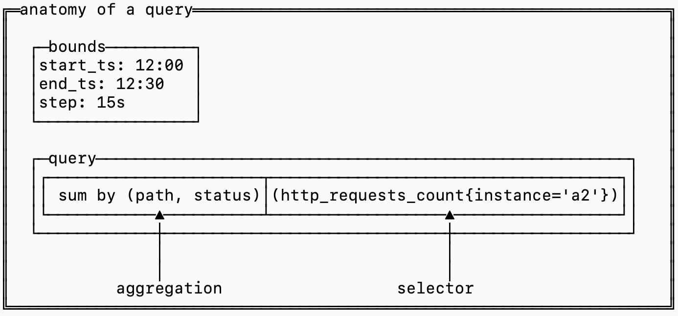
The selector determines which series should be fetched and included in the query while the aggregation defines the logic for combining together samples across different series.
Think about it like a 2D matrix where each series is a row and each timestamp is a column. The cells hold the measurements at each timestamp.
Efficiently computing the query requires figuring out how to prune series to only the series matched by the selector, extracting the samples for the time range needed, grouping them by the aggregation and finally computing the results.
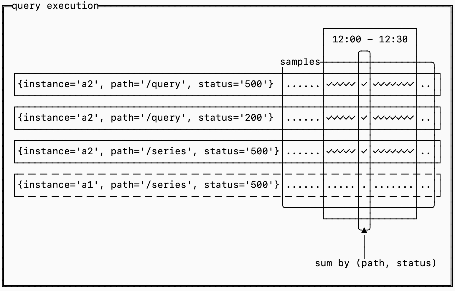
This is done in three steps:
An inverted index is used to narrow down which series need to be fetched
A forward index determines which series need to be aggregated together
The raw samples are retrieved and aggregated
the inverted index
The query starts here. The inverted index narrows down potentially hundreds of thousands of series into just the ones required to serve the query.
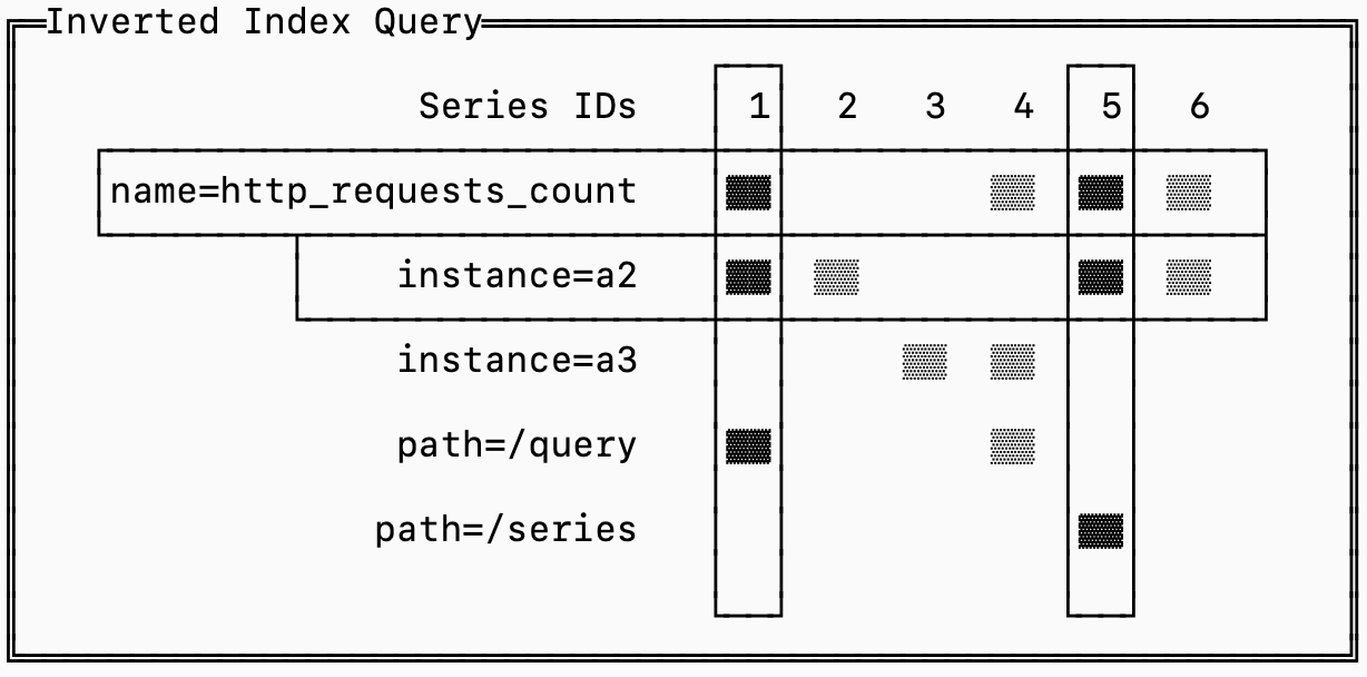
For example the query http_requests_count{instance='a2'} needs to fetch all the series for http_requests_count that also have the label instance=’a2’ and can ignore the rest.
A naive approach is to store series sorted by name. That would allow us to binary search the entire database to isolate only series with the name http_request_count and then scan those to find which belong to instance='a2'.
The problem is that there may be thousands of instances, each collecting hundreds of metrics, so narrowing down the set to just series that match instance=’a2’ isn’t trivial.
The solution to this problem is borrowed from search systems: the inverted index.
For every label that exists, the database stores a list of the series that have that label. This list is called a “posting list”.
Finding the requires series is reduced to an intersection of posting lists.
To make this intersection efficient, each series is assigned a unique ID and the posting lists are sorted by this ID. That makes the algorithm simple: you load the posting lists for the labels you care about and advance pointers into the lists until they all align on a series ID, that’s one you need to fetch (in the diagram above, series 1 and 5). You continue until you’ve exhausted one of the posting lists and you can ignore posting lists that aren’t part of your query.
roaring bitmaps
There are some encoding tricks you can use to store and leverage the inverted index efficiently. The state of the art mechanism for this particular use case is called a roaring bitmap.
The insight with this data structure is that posting lists tend to be either sparse or dense, and the sparse ones tend to be clustered. For timeseries, you can imagine that the posting list for container_id=123 (a sparse list) holds significantly fewer series than region:us-west-2 (a dense list). If you assign series ids monotonically, though, it’s likely that all the series generated by container_id=123 have ids within a small range of the total series id domain (they all get registered on startup).
To leverage this observation, roaring bitmaps split the representation of posting lists into “dense blocks” and “sparse blocks”. Since they only encode 32-bit integer values, they index these blocks by the “high 16” bits and then the blocks encode which exact values exist. Dense blocks encode bitsets to represent which values are present while sparse blocks just encode the array of values naively.
In the example below, we have representations for both sparse and dense blocks. The sparse block encodes the values [5, 1000] while the dense block encodes every number between 196608 and 250000.
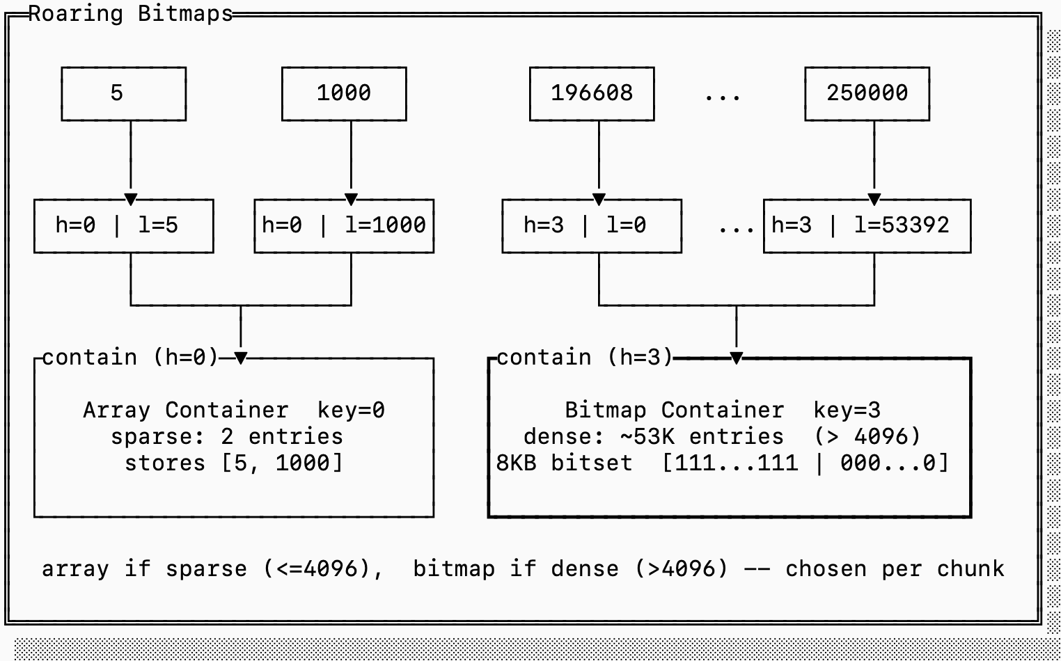
If we were to encode the sparse block with a full bitset it would take 8KB since we need one bit for every value that starts with 0x0000. But since there are only two numbers, it’s more efficient to just encode 4 bytes (the lower 16 bits for each 5 and 1000).
On the other hand if we were to encode the dense block as a simple array, it would require 212KB (2 bytes per entry). It’s more efficient to store a single 8KB bitset.
Roaring bitmaps are not only efficient in storage space. Because the lists are sorted, and because bitmap intersections/unions can be done with SIMD instructions, set operations on roaring bitmaps are incredibly efficient.
the forward index
If you followed the inverted index section closely, you’ll notice that we made a small decision with big implications: the inverted index only stores series ids not the series definitions themselves.
This means that while the inverted index helped us find which series IDs we need to serve a query, it doesn’t help us at all for determining which series should be grouped together for an aggregation.This means we need some mapping of series IDs to their definitions (the label set).
This is called the forward index:
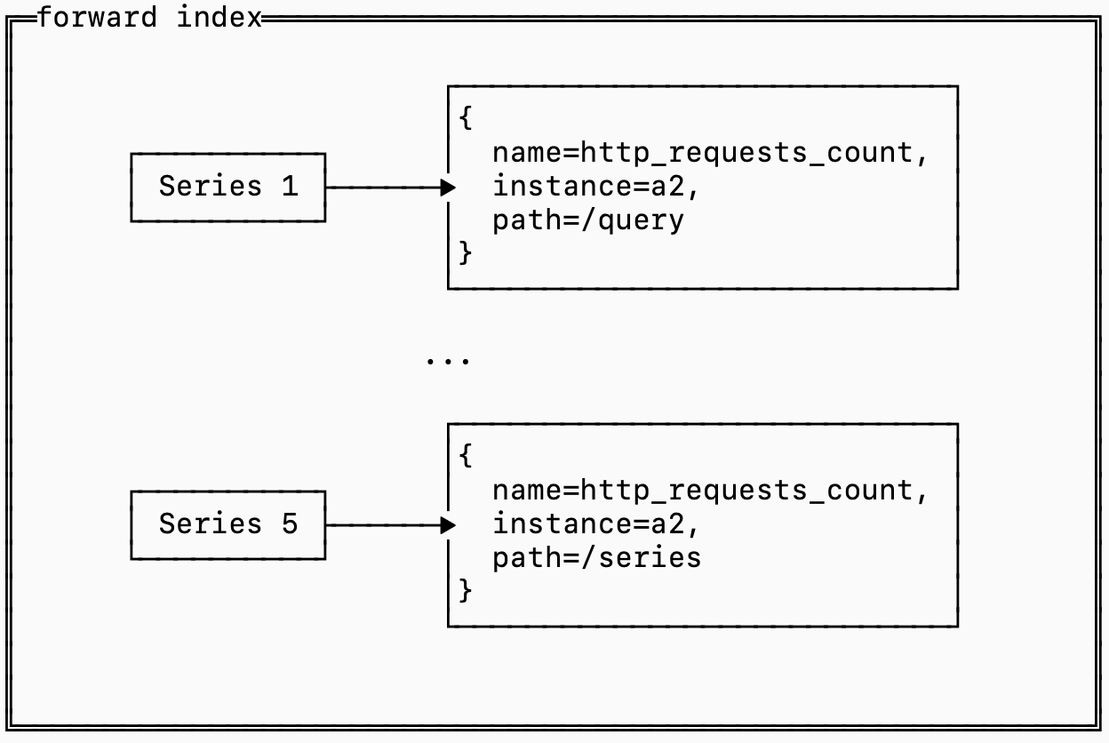
Since queries need to load the forward index for every series it matches, the retrieval of this data can get expensive.
Most data that is stored on disk, including indexes like the forward index, is stored in something similar to an SST (see this previous post on that for more detail), which means you choose a key that you sort by. This is called the “clustering” key, and how you choose it makes a big difference to your storage performance.
To make this concrete, here are two alternative layout options for storing series and forward indexes:
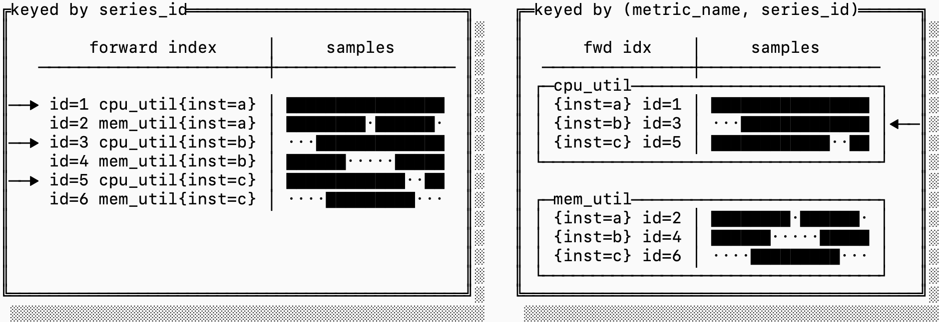
In the first example, we just choose to sort by series_id. This makes it easy to go from the inverted index to then retrieve the samples and the forward index because each posting in the inverted index is just the series ID.
The problem is that series IDs have no encoding or relationship to the metric name. If a query targets only a specific metric (which is the case for almost every query), it may have to fetch series that are scattered on disk, which can dramatically increase the read amplification of a query.
The layout on the right sorts the forward index and samples based on a composite key of (metric_name, series_id) instead. This means that consecutive series IDs are not necessarily clustered, but blocks on disk are dedicated to a single metric. If you need to fetch many series for the same metric, this can be significantly more efficient.
storing samples
Now that we have a way to know which series we need and which ones group together in an aggregation, we just need a mechanism for storing and fetching the raw data.
An interesting observation is that timeseries data is both abundant and repetitive, a combination that results in some interesting characteristics that make it particularly amenable to compression (something we discussed in depth in a previous post).
A data point in a series, called a sample, has two parts: the timestamp the measurement was taken and the value of the measurement.
timestamps
If you’ve ever configured prometheus, you know that you configure your scraper to scrape at some regular interval (perhaps every 15s). That means it shouldn’t surprise you when the timestamps in any particular series look a lot like this:
┌series A timestamps────────────────────────────────────┐
│┌────────┐┌────────┐┌────────┐┌────────┐     ┌────────┐│
││00:00:00││00:00:15││00:00:31││00:00:45│ ... │01:00:00││
│└────────┘└────────┘└────────┘└────────┘     └────────┘│
└───────────────────────────────────────────────────────┘
You may occasionally see gaps that are wider (e.g. if a pod is overloaded), but in stead state you expect the timestamps to always be ~15s apart.
The typical encoding of a timestamp is an i64 long, which takes up 8 bytes. If you were to encode 100k series every 15s that would take you 192 MB/hour just to store timestamps. In production, however, most systems are able to store this with just ~3 MB/hour (a 60x reduction). How?
Some smart people figured out that if you store only the first timestamp, and then encode just the difference between them, you can store these points using much less data:
┌─series A timestamps (deltas)────────────────────────────┐
│ ┌────────┐┌────────┐┌────────┐┌────────┐     ┌────────┐ │
│ │00:00:00││00:00:15││00:00:31││00:00:45│ ... │01:00:00│ │
│ └────────┘└────────┘└────────┘└────────┘     └────────┘ │
│     ┌────────┐ ┌────────┐ ┌────────┐                    │
│     │  15s   │ │  16s   │ │  14s   │ ...                │
│     └────────┘ └────────┘ └────────┘                    │
└─────────────────────────────────────────────────────────┘
Using 2 bytes per delta, you can encode up to gaps of 18 hours (65k seconds) and reduce your overall data by 4x.
Because the timestamps are reported at 15s intervals, It turns out we can do even better. The difference of the difference between timestamps is even smaller, in fact it’s almost always pretty close to 0.
┌series A timestamps (delta of deltas)───────────────────┐
│┌────────┐┌────────┐┌────────┐┌────────┐     ┌────────┐ │
││00:00:00││00:00:15││00:00:31││00:00:45│ ... │01:00:00│ │
│└────────┘└────────┘└────────┘└────────┘     └────────┘ │
│    ┌────────┐ ┌────────┐ ┌────────┐                    │
│    │  15s   │ │  16s   │ │  14s   │ ...                │
│    └────────┘ └────────┘ └────────┘                    │
│          ┌────────┐ ┌────────┐                         │
│          │   1s   │ │  -2s   │                         │
│          └────────┘ └────────┘                         │
└────────────────────────────────────────────────────────┘
There are some fancy ways that you can encode deltas of deltas so that you can store timestamps in approximately 1 bit per sample, a 64x reduction from the original 8 byte format.
measurements
If you got the gist of the last section, you may have already deduced that measurements might follow a similar pattern. Metrics typically change slowly over time (unless something special is happening, which by definition doesn’t happen often).
This sound pretty similar to what we saw when we were discussing timestamps, but the problem is that a measurement is a floating point value. A small difference between two floating point numbers can still require many bits.
Take for example the IEEE 754 (the standard) representation for 0.0001, such a simple decimal surprisingly looks like this:
0011111100011010001101101110001011101011000111000100001100101101 ┌────────────────────┬────────────────┬───────────────────┐
│ Component │ Bits │ Value │
├────────────────────┼────────────────┼───────────────────┤
│ Sign (1 bit) │ 0 │ + │
├────────────────────┼────────────────┼───────────────────┤
│ Exponent (11 bits) │ 01111110001 │ 1009 − 1023 = −14 │
├────────────────────┼────────────────┼───────────────────┤
│ Mantissa (52 bits) │ 1010...0101101 │ fractional part │
└────────────────────┴────────────────┴───────────────────┘The sign bit is simple (positive or negative). The mantissa is multiplied by 2 ^ exponent to recreate the fractional value, in this case we get:
(−1)^0 × 1.1010...0101101₂ × 2^−14 ≈ 0.00010000000000000000479That’s not exactly 0.0001 but it’s as close as we can represent with floating point numbers. The interesting thing is that you might notice that 0.0001 and 0.0002 look… very similar (in fact, the mantissa is the same):
  ┌────────┬──────┬─────────────┬────────────────────────────┐
  │ Value  │ Sign │  Exponent   │  Mantissa                  │
  ├────────┼──────┼─────────────┼────────────────────────────┤
  │ 0.0001 │ 0    │ 01111110001 │ 101000110110111...00101101 │
  ├────────┼──────┼─────────────┼────────────────────────────┤
  │ 0.0002 │ 0    │ 01111110010 │ 101000110110111...00101101 │
  └────────┴──────┴─────────────┴────────────────────────────┘
If you XOR these two values you get a value with a lot of 0s:
0000000000110000000000000000000000000000000000000000000000000000This isn’t coincidence, many similar floating point numbers have lots of 0s when you XOR them. This means you can store a three part number: first store the number of leading 0s (10) then store the meaningful length (2) then store the meaningful bits 0b11 which is only 2 bits. This takes you down from the original 64 bits to just 15 bits (in this case).
Together these two concepts (delta of delta encoding for timestamps and XOR encoding for measurement values) allow us to store many measurements extremely efficiently, storing on average only ~11 bits per measurement, down from 16 bytes of the naive format.
Going back to our original 100k series reported at 15s interval, you go from 384 MB/h to 33 MB/h, a nearly 12x improvement.
series churn
Let’s revisit the 2D matrix model of timeseries where the horizontal dimension is time and the vertical dimension are the series. If you look at a few hours of production data you would probably see something like this:
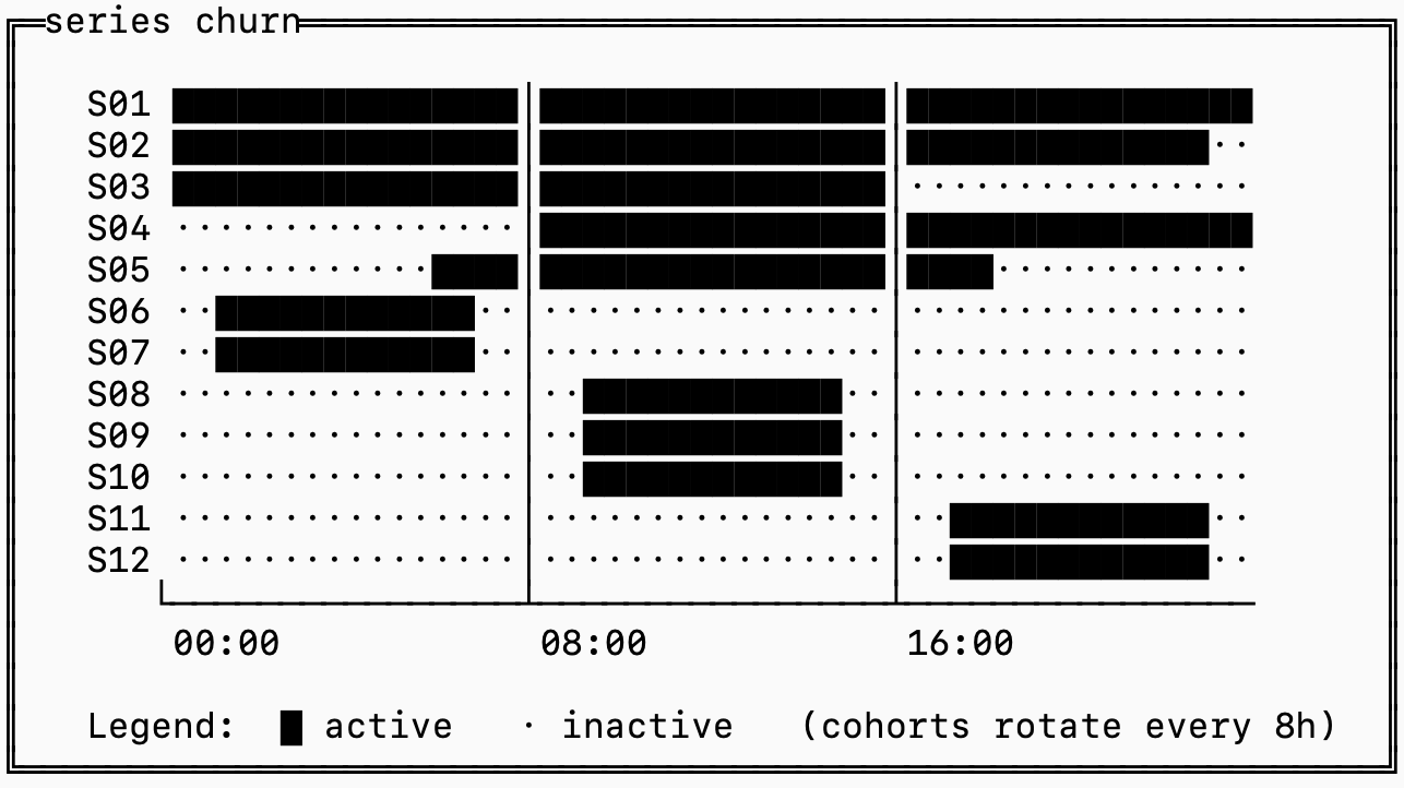
The ██ represents series with data during that time and a . represents series with no data at that time.
Series S06-S12 are likely tagged by something like container_id that is not static, so whenever you deploy a new series is generated with nearly identical labels except for a change in container_id.
This is called “series churn”, and it’s the biggest problem in timeseries databases. If we were to ignore this pattern in observability systems, we’d end up with some pretty nasty side effects.
For illustration, imagine there were only 2 labels on each of these metrics: name (the metric name) and container_id. If we indexed this in a single inverted index you’d see something like this:
name=metric_1: [1, 3, 5, 7, 9, 11]
name=metric_2: [2, 4, 6, 8, 10, 12]
container=a:   [1, 2, 3]
container=b:   [4, 5]
container=c:   [6, 7]
container=d:   [8, 9, 10]
container=e:   [11, 12]
If my query targeted the time range 16:00-24:00, and I’m querying for metric_2 then I’d need to examine all of [1, 3, 5, 7, 9, 11] because that’s the only filtering condition I have. I would then discover that series [7, 9] don’t have any data associated with the window I’m querying, but only after I’ve fetched the samples for those series.
The solution to this is bucketing: storing a full trio of samples, inverted and forward indexes for each “bucket” of time. The series IDs are also scoped to a bucket, which allows you to quickly find the series ID for incoming data without looking through the entire history of series.
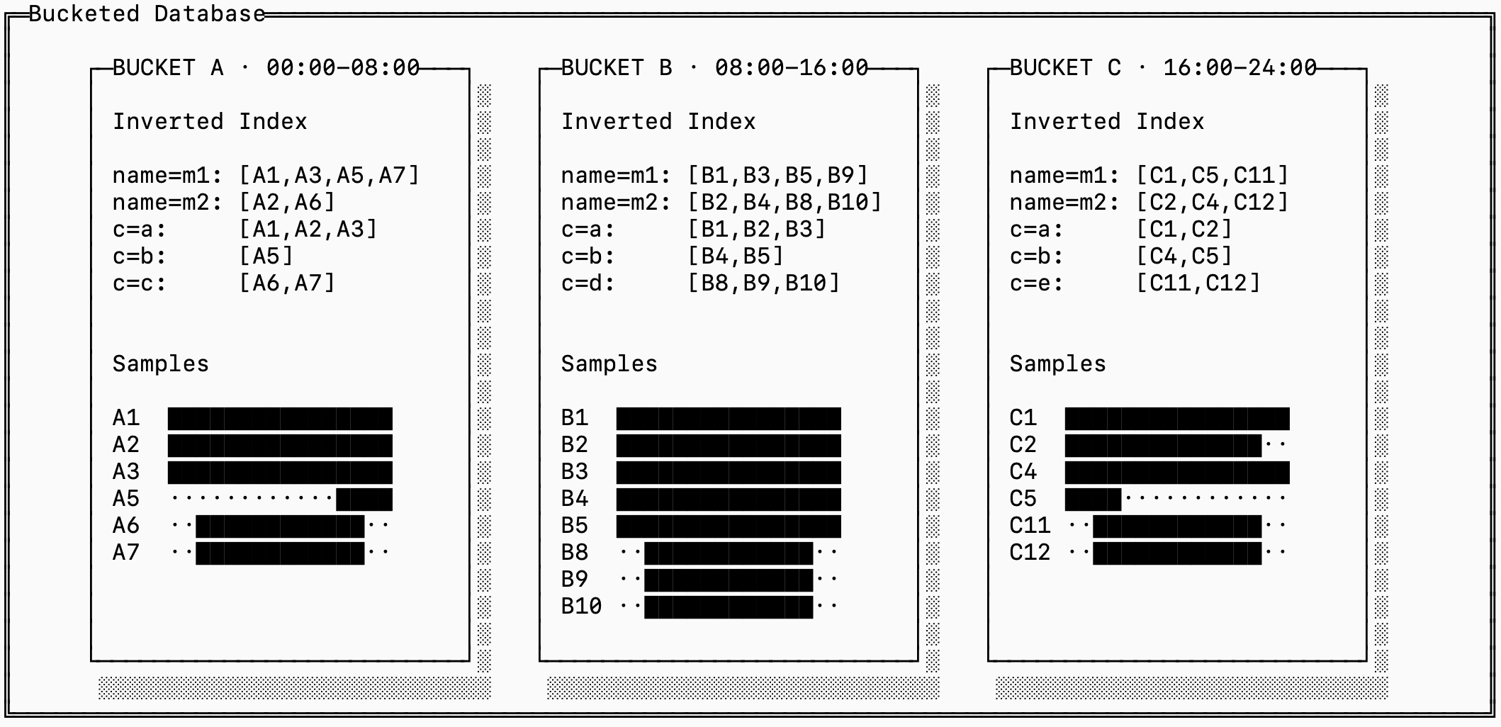
Notice that the downside of this is that this generates many more distinct series IDs, even though some of them refer to the same “logical” series. In the example above, A1, B1, and C1 all have the same labels.
This is a fundamental tradeoff between read, write and space amplification in timeseries storage. You can manage this by merging series across time blocks together for older buckets, and this is in fact exactly how many timeseries databases handle the problem.
fsync()
That’s it for today! If you want to read up more details on how we encode and store these data types on disk, we have a detailed RFC on GitHub.
We’ve covered the three main types of data that a timeseries system stores: samples, inverted indices and forward indices as well as how they are represented on disk. Coming soon, I’ll write a full post on the query execution pipelines for timeseries engines so make sure to subscribe to get it delivered straight to you.
I love every single post on this blog. I can tell a lot of heart and soul went into it.
This was a great post Almog I learned a lot!