

the mathematics of compression in database systems
why compression is (almost) always worthwhile

This post is a little departure from our usual architecture discussions, but I promise it is worth understanding if you care about your database performance.
I started thinking about compression when implementing prefix compression for SlateDB. When I ran benchmarks, I noticed that performance seemed "worse" despite improved compression ratios.
This got me thinking deeper about why databases use compression, and what the right framework is for reasoning about whether that tradeoff is worth it. This post is the result of that exploration, and I hope it helps you understand why, when and how data systems use techniques to reduce data size.
understanding “compression math”
The first rule to understand about why compression is important is that there are effectively three resources that databases can be bottlenecked on1:
I/O Bandwidth: bytes/sec from disk, network, or even DRAM into your CPU caches
CPU: cycles available on your machine for processing
Memory: transient storage that is orders of magnitude faster to access than disk/network
Compression gives you a knob to tune between these resources. More specifically, compression directly trades I/O for CPU because it takes CPU cycles to compress and decompress data but moving compressed data requires less I/O bandwidth.
Mathematically, we can reason about this tradeoff by computing the cost of compression and applying it to different resource utilization. Let’s assume for a given workload and compression we have the following properties2:
is compression about latency?
Naively, we can compute a hypothetical breakeven I/O bandwidth β that determines whether compression will speed up a point-to-point transfer.
An uncompressed data transfer takes S/B_x seconds. Compressing then transferring the same dataset takes T_c + S_c/B_x + T_d seconds3, since you first need to compress the data before sending it and decompress it after sending it. In other words, compression improves the overall transfer latency when:
Using this we can compute our breakeven bandwidth:
To make this concrete I timed the (de)compression of a sample data taken from a compression challenge with a baseline of 191MiB using both zstd level 4 (fast, lighter compression) and level 10 (slower, more aggressive compression):
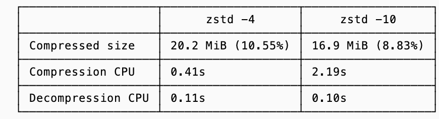
Using the breakeven formula from above, the breakeven points for compressing the data are 328 MiB/s (2.76 Gbps) and 76 MiB/s (0.64 Gbps) for levels 4 and 10 respectively.
An r5d.xlarge instance has baseline B_network of 1.25 Gbps, meaning if latency is all you cared about zstd with level 4 compression is worthwhile but level 10 is not: the improved compression is overshadowed by the time it takes to achieve it.
The very same instance, however, has a speedy NVMe disk with B_NVMe of 10s of Gbps. This would make it seem like if you aren’t transferring data over the network, you shouldn’t compress with either of these options! And if your only bottleneck were the latency of a one-shot transfer from disk into the CPU, that conclusion would be right… but the breakeven analysis assumes the I/O pipe is otherwise idle, which is rarely true in a database.
saturation and the CPU ↔ I/O exchange rate
In practice, databases are not doing one-shot transfers of a blob from disk to RAM and calling it a day. Instead, they need to constantly read significant amounts of data to handle incoming requests, compress old files, fill caches, etc. Put another way, databases will saturate their I/O bandwidth much before they saturate CPU. Sustained throughput matters far more than latency.
Instead of thinking about a breakeven latency point, we can think about compression as a way to exchange bandwidth for CPU. I’ll refer to the effective throughput after accounting for compression as logical bandwidth:
Getting back to our example from before, zstd level 4 gives us ~9.4x compression ratio. This means that our logical bandwidth on a 1.25 Gbps network line is 11.75 Gbps. Put another way, we can sustain a throughput of 11.75 Gbps if we compress/decompress as compared to 1.25 Gbps if we send raw data over.
Of course, this logical bandwidth only materializes if you can afford the CPU cost. A useful way to think about codecs is in terms of (de)compression throughput θ:
To fully saturate a pipe of bandwidth B_x you need:
In other words you need to be able to compress data faster than you can send it over the network.
This math starts to influence decisions when you look at the increasing amount of time it takes for rather trivial improvements at higher levels of compression (for the same 191MiB dataset from before):
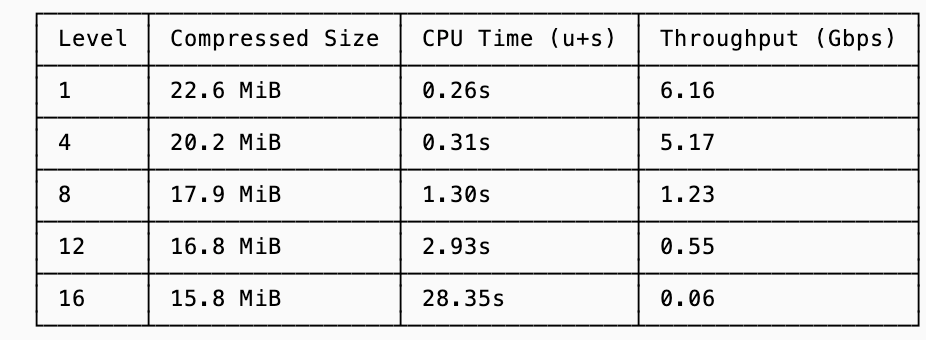
There’s an obvious diminishing return of the higher compression levels, and this is why databases don’t simply choose to use the most aggressive compaction. But we can go one step further and put a dollar value to the exchange rate between CPU and logical bandwidth.
putting a dollar value on compression
The final principle to consider when evaluating whether (and how aggressively) to compress is in the context of managed services that markup their cost per byte, meaning they put an artificial premium on bytes that make compression even more valuable. The typical example here are egress and ingress fees with cloud providers.
This ends up looking quite similar to the exchange rate between CPU and I/O, except instead you are trading CPU for dollars. Let’s consider the r5d class of instances on AWS; you’ll have the following rates:
$0.072 / vCPU hour (in
us-west-2)$0.02 / GB transferred across zones (ingress + egress)
Using these numbers, sustaining 1 Gbps of physical bandwidth (450 GB/h) costs $9/hour in transfer fees alone. To sustain 1 Gbps of logical (uncompressed) throughput, you only need to transfer 1/R Gbps on the wire, so your bandwidth cost drops to $9/R per hour. But to get this you need enough CPU to compress at that rate. Since θ measures how many Gbps a single vCPU can compress, you need 1/θ vCPUs to keep up. At $0.072 per vCPU-hour, your total cost to sustain 1 logical Gbps is:
In other words, you pay less GB transfer costs the higher your compression ratio is but to achieve a higher compression ratio and sustain that throughput you need to pay more CPU. Plugging in the table of observed values from the previous section:
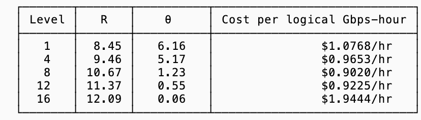
For these particular compression ratios, choosing zstd level 8 is your best bet (if what you care about is reducing cost).
sometimes it is about latency
Bringing it back to where we started, it’s often worth being conservative about compression levels. While the cost equation above suggests that something like zstd level 8 minimizes dollars per unit throughput, databases don’t live entirely in the world of steady-state bandwidth.
In many systems, decompression happens directly on the query critical path. In those cases, every additional millisecond of extra CPU time can show up in tail latencies, and the most cost-efficient compression level may not be the latency-optimal one.
One useful property (see the data in the latency section) is that decompression time is nearly constant across levels. The CPU cost asymmetry is heavily skewed toward the write path. This means you can invest in aggressive compression at write time where latency is often more tolerable without penalizing read-side tail latencies. The practical implication is that for write-once, read-many workloads, the compression level decision is primarily a write-path throughput question.
As with all things databases, these are tradeoffs you need to make with your workload and preferences in mind.
consider getting hands on
Before I get into the techniques used, I often feel the best way to learn about performance optimizations (including data size) is to play around with them yourself. To that end, I created a challenge to compress a sample dataset of one million rows as much as possible. The naive dataset serialized as JSON is 210MB, zstd at level 22 gets down to 11MB, and after a few hours of bit twiddling I got it down to 9.4MB.
I’m maintaining a leaderboard, so you can try your hand at the challenge yourself: https://github.com/agavra/compression-golf
In addition, there are some interesting submissions that detail their approaches to compressing the dataset (typically as comments at the top of the file or in the PR they submit). You may want to start by reading this blog, and then applying that understanding to understand the leading submissions.
techniques for data reduction
There are two main techniques for reducing data size:
Semantic Encoding: these techniques understand the data patterns and change the binary representation to be more compact. Examples include prefix, varint and run-lenght encoding (discussed more later).
Entropy Compressors: these have no knowledge of the data semantics, but they can analyze the bytes to find redundancy and then use various techniques to reduce the entropy. Examples include zstd, snappy and gzip.
These two techniques are often applied together. First you will use semantic encoding to reduce your logical data size, and then apply entropy compression to further compress the data.
Entropy compression alone gets you pretty far. On the compression golf dataset, zstd -9 took 210MB down to 18MB (level 22 reached 11MB). Adding standard semantic encodings got us to 7MB with the most aggressive techniques getting down to 5MB.
The more important property is the CPU cost. Since semantic encodings are mostly O(n) passes with simple ops they are cheap to run. If you apply them first your entropy compressor has less (and lower entropy) data to chew on, requiring fewer CPU cycles.
Connecting this back to the cost model shows how this two-layer compression pays dividends. On the compression-golf dataset, my semantic codec reduced the data from 191 MiB to ~11 MiB. Applying zstd on top brought it down to 7.2 MiB in a total of 1.4s, which is comparable CPU time to zstd level 8 alone (1.3s) but with 2.5x better compression.
Plugging this into our cost formula computes θ ≈ 1.14 Gbps (similar to level 8) and R ≈ 26.5 (vs 10.67 for level 8). Since the bandwidth term $9/R dominates the cost equation, that ratio improvement is dominating bringing the total cost to $0.40/hr per logical Gbps, less than half of the previous best (see cost table in the section on dollar value of compression).
Entropy compression techniques are well explored4 and can be applied to your data with little to no modification from you. There are many libraries (zstd, gzip, snappy) that implement entropy-based compression you can pick up off the shelf and apply to your workload. Since it is unlikely you will need to implement any of these techniques yourself, the rest of this post will focus on how you can apply semantic encoding to your data.
small encodings of common datatypes
There are standard, in-memory byte representations for many data types that I suspect you are familiar with.
An example of this is u32 (an unsigned5, big-endian, 32-bit integer). For example the number 2,031,620 is represented like this:
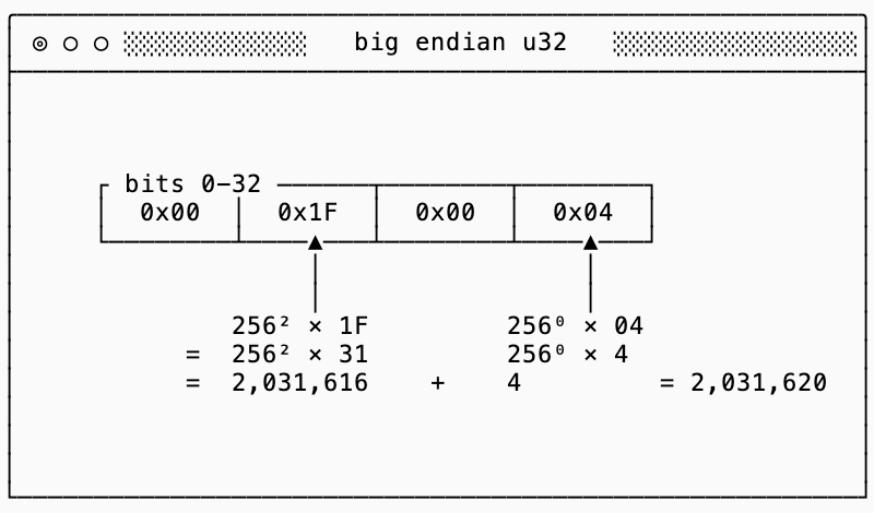
Each of the four bytes (in this case represented as hexadecimal codes) represent orders of magnitude more significant values than the next (by a factor of 256, the number of values that each hex code can represent).
If we were to store these as bytes (on disk, in memory, etc…) each one takes up 32 bits. If I store 1024 of these u32 integers I’m storing 32KB of data. Can we do better?
Turns out when you have a u32 field, most values are typically pretty small and the first and second byte would both be 0x00. To avoid storing unnecessary 0x00 bytes on disk, there are strategies such as variable encoding that will use the most significant bit to indicate whether or not more bytes are needed past the current byte (and then the remaining 7 bits to store data).
Here is an example of encoding the same integer as above, but using only 3 bytes. Note that we need to encode the least-significant bytes first (little endian encoding) so that we can stop as soon as we no longer need more bytes.
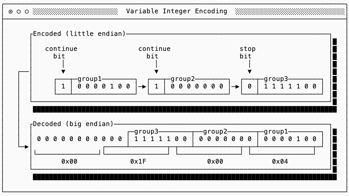
This gets more efficient the smaller the numbers are. Numbers less than 128 only take 1 byte!
My favorite characteristic of varint encoding is that there is no size limit, you can encode a u16, u32 and u64 all with the same encoding. This makes it backwards compatible to change the in-memory representation (upcast from a four byte to eight byte integer) without changing the underlying storage and is a technique used by many formats such as Parquet and Protobuf.
There are various other strategies that help achieve similar results for other data types, but varint is the most common of them.
delta, run-length, prefix and XOR encoding
The next class of techniques exploit the fact that in-memory types are more general than necessary. This makes sense for mutable data since you need headroom for values you haven’t seen yet. Once the data set is fixed (on disk, for example) you can examine it and choose tighter encodings.
Each of these four techniques help take advantage of the observation that data is typically sorted or clustered in a way where similar values are next to one another.
I’ll summarize these techniques below and help you with understanding when each should be chosen but for the full algorithms there are various more detailed explanations online:
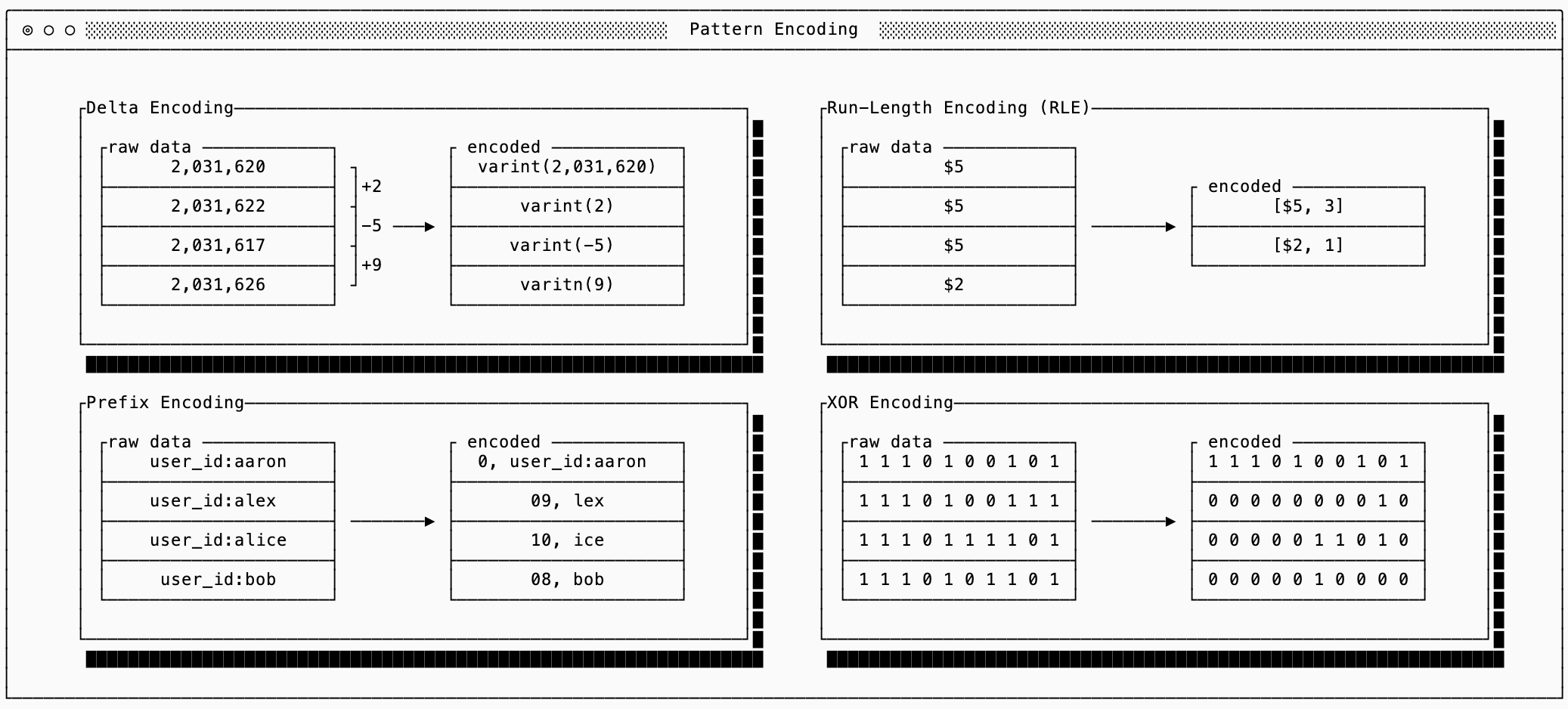
Delta: use when integers are semantically close to one another. Instead of encoding the raw values, encoding only the first raw value and then the differences (deltas) between them. Often the deltas will be much smaller than the raw data, allowing varint encoding to work better than it would on the raw numbers.
Run-Length Encoding (RLE): use when there are many repeated values or sparse data. When many values repeat, encode the value once and then the number of times it repeats. This is commonly used in columnar data formats.
Prefix Encoding: use with sorted strings. Since sorted strings often share prefixes you only need to encode the length of the shared prefix and the suffix. Combined with Delta encoding or RLE you can reduce the size of the encoded prefix lengths.
XOR Encoding: use mostly for similar floating point values. This is similar to Delta encoding, but sometimes a small difference between floating points requires a ‘large’ representation. It works by XOR’ing the bits, so values that are similar to one another will typically end up with many 0s. There are then techniques you can use (see Gorilla for example) for compressing values that are sparse.
dictionary encoding
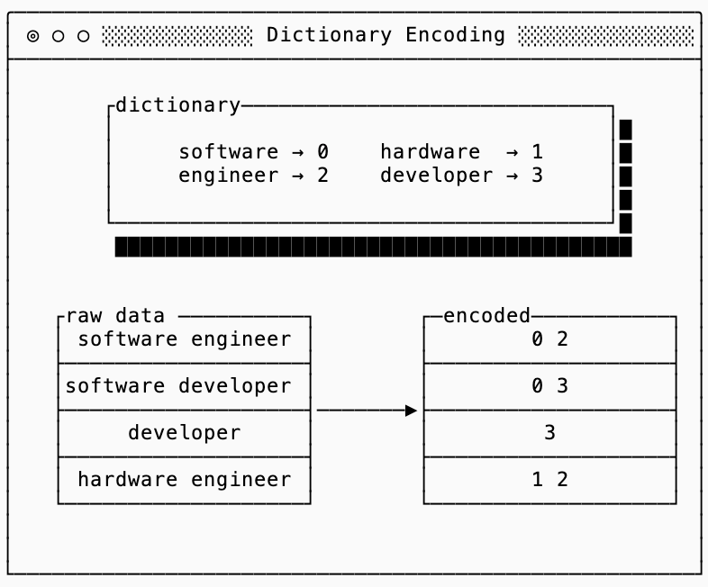
Dictionary encoding helps when you have repeated data (or data patterns) that aren’t necessarily close in proximity, meaning you can’t use one of the techniques previously discussed. In other words, the word “engineer” might show up frequently in a database of users as the job title but not next to users that are near one another.
To solve this, dictionary encoding is a technique that maps commonly used tokens to numeric identifiers, and then replaces the tokens with the identifier themselves. There are many ways to represent the dictionary concisely (FST, Front Coded Lists, Radix/MARISA Tries, etc…) depending on the data distribution and requirements, but the main concept remains the same.
The interesting thing about dictionaries is that they’re often used by entropy-based compressors (such as zstd) because they can see repeated sequences of byte strings. This means that using a semantic dictionary alone is not very useful if all you care about is compressed data size, you’re just repeating work that your compressor is going to do anyway.
The benefits of the dictionary are second order.
First, semantic dictionary encoding is faster because it can add a string to a dictionary as soon as it encounters it. In the meantime an algorithm like zstd needs to consider all possible sequences of bits and doesn’t know which ones repeat without a complicated lookback mechanism.
Second, it unlocks other encodings (like delta encoding and bitpacking), which compounds to improve the overall compression ratio.
bit-packing
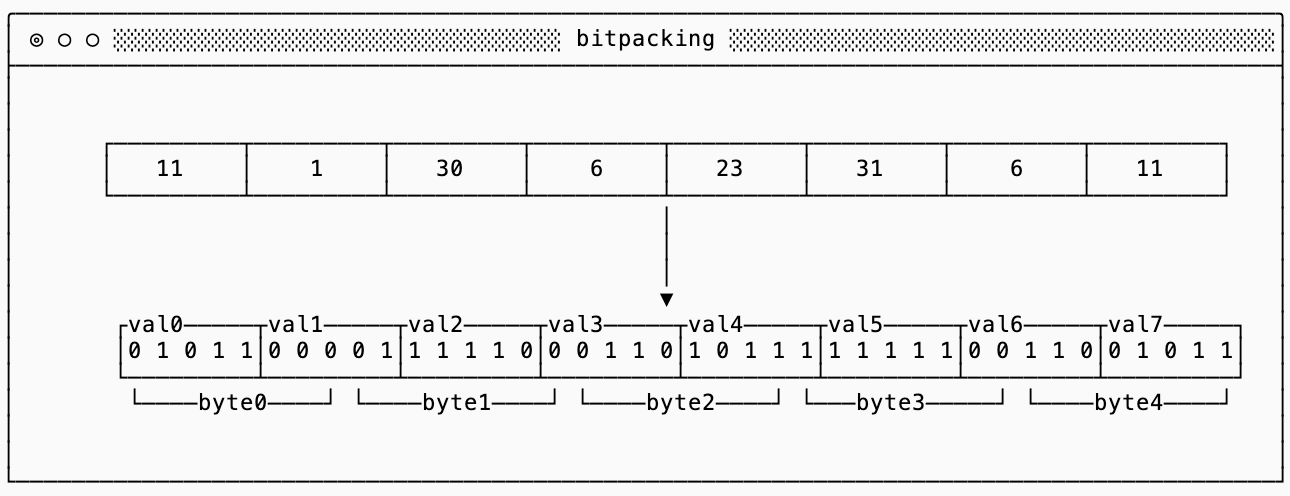
Bitpacking is a technique used to ignore byte-alignment and pack multiple values into a single byte. A classic example of bit-packing is to pack eight boolean values into a single byte, using just one bit to represent each boolean.
The technique extends to more complicated data types as well. For example, if you know that deltas between all of your values are between 0 and 32 you only need 5 bits to represent each delta. The smallest varint is still 1 byte (8 bits), so you can do even better if you pack eight 5-bit values into 5 bytes:
You should use bitpacking with extreme caution.
Not only is it easy to get your encodings wrong, but it can cause your final compressed dataset to be larger than if you hadn’t bitpacked. This is because most entropy-based compressors (zstd included) are byte-aligned, meaning they look for repetition along byte boundaries. If you have many repeated 7-bit strings the data looks “scrambled” to the eyes of a byte-aligned algorithm, so it won’t be able to do its job properly.
To show this I ran a quick experiment (see code and full results) that generated 10k values between 0 and 127 (values that fit in 7 bits), sorted them and then compared the final compressed size if I were to just use full 8-bit values or if I bitpacked them into 7-bit values.
Despite the bitpacked representation being smaller before compression (8,750 bytes vs 10,000 bytes), zstd compresses the raw bytes down to just 246 bytes, which is nearly 3x better than the 662 bytes it achieves on the bitpacked version.
lossy compression
The techniques described earlier in this blogpost are all “lossless”. In other words, you can reconstruct the exact dataset you compressed initially. Sometimes, though, you can accept a lossy compression. Most of these techniques are domain-specific, and you are probably familiar with this concept in image and video processing.
While these techniques are interesting in their own right, I’ll save covering them for a future post (stay tuned for a post on vector databases, which leverage lossy compression quite elegantly).
fsync()
And we’re done for today! If you take away just one thing from this post it should be that compression is (almost) always worth doing, but how much compression depends on certain parameters of your workload.
If you read my post on database foundations, you might see some parallels with the RUM conjecture here.
All measurements in this blog post use CPU time, not wall clock time, when evaluating compression. I had originally attempted using valgrind to count the number of CPU instructions, but (a) this made some heavier compression algorithms take over thirty minutes to run and (b) the conversion from CPU instruction to time depends on the IPS (instructions per second) which depends on the instructions and not the clock speed.
You can use streaming compression algorithms to pipeline/stream compressed data, which makes the story for compression even more compelling since you can concurrently serialize, transfer and deserialize packets.
See techniques like Huffman Encoding and Entropy Coding, or look at implementations of systems like zstd.
Signed numbers are a little trickier to deal with because the standard two’s complement encoding uses the first bit to indicate that a number is negative. This means you need all the bytes to know whether a value is positive or negative. There are alternative encodings, the most popular is zigzag, which help solve this problem.
Really enjoyed this, especially the framing of compression as a tradeoff between CPU and I/O rather than just “making things smaller.” That perspective feels a lot closer to how systems actually behave under load.
The layering you described also stood out to me. The idea of doing some form of semantic or structural encoding before entropy compression feels like where a lot of untapped potential is. Most systems seem to stop at entropy, even though reshaping the data beforehand could reduce the problem space significantly.
I’ve been experimenting with something similar on a smaller scale, trying to push compression slightly closer to structure and meaning instead of just pattern detection. Not replacing something like gzip or zstd, but giving them a cleaner input to work with.
One thing I’m curious about is how you think about the boundary between semantic encoding and complexity. At what point do the gains start getting outweighed by the cost of generalizing across different types of data?
It feels like that edge is where most of the interesting work is right now.